Exercise: PCA in 2D
2014-09-14 20:41
387 查看
Step 0: Load data
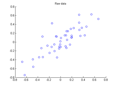
The starter code contains code to load 45 2D data points. When plotted using the scatter function, the results should look like the following:
Step 1: Implement PCA
In this step, you will implement PCA to obtain xrot, the matrix in which the data is "rotated" to the basis comprising

made up of the principal components
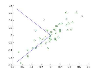
Step 1a: Finding the PCA basis
Find

and

, and draw two lines in your figure to show the resulting basis on top of the given data points.
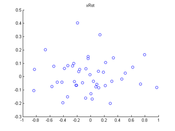
Step 1b: Check xRot
Compute xRot, and use the scatter function to check that xRot looks as it should, which should be something like the following:
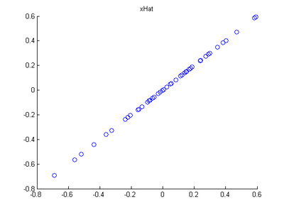
In the next step, set k, the number of components to retain, to be 1
Code
The starter code contains code to load 45 2D data points. When plotted using the scatter function, the results should look like the following:

Step 1: Implement PCA
In this step, you will implement PCA to obtain xrot, the matrix in which the data is "rotated" to the basis comprising
made up of the principal components
Step 1a: Finding the PCA basis
Find
and
, and draw two lines in your figure to show the resulting basis on top of the given data points.

Step 1b: Check xRot
Compute xRot, and use the scatter function to check that xRot looks as it should, which should be something like the following:

Step 2: Dimension reduce and replot
In the next step, set k, the number of components to retain, to be 1

Step 3: PCA Whitening

Step 4: ZCA Whitening

Code
close all
%%================================================================
%% Step 0: Load data
% We have provided the code to load data from pcaData.txt into x.
% x is a 2 * 45 matrix, where the kth column x(:,k) corresponds to
% the kth data point.Here we provide the code to load natural image data into x.
% You do not need to change the code below.
x = load('pcaData.txt','-ascii'); % 载入数据
figure(1);
scatter(x(1, :), x(2, :)); % 用圆圈绘制出数据分布
title('Raw data');
%%================================================================
%% Step 1a: Implement PCA to obtain U
% Implement PCA to obtain the rotation matrix U, which is the eigenbasis
% sigma.
% -------------------- YOUR CODE HERE --------------------
u = zeros(size(x, 1)); % You need to compute this
[n m]=size(x);
% x=x-repmat(mean(x,2),1,m); %预处理,均值为零 —— 2维,每一维减去该维上的均值
sigma=(1.0/m)*x*x'; % 协方差矩阵
[u s v]=svd(sigma);
% --------------------------------------------------------
hold on
plot([0 u(1,1)], [0 u(2,1)]); % 画第一条线
plot([0 u(1,2)], [0 u(2,2)]); % 画第二条线
scatter(x(1, :), x(2, :));
hold off
%%================================================================
%% Step 1b: Compute xRot, the projection on to the eigenbasis
% Now, compute xRot by projecting the data on to the basis defined
% by U. Visualize the points by performing a scatter plot.
% -------------------- YOUR CODE HERE --------------------
xRot = zeros(size(x)); % You need to compute this
xRot=u'*x;
% --------------------------------------------------------
% Visualise the covariance matrix. You should see a line across the
% diagonal against a blue background.
figure(2);
scatter(xRot(1, :), xRot(2, :));
title('xRot');
%%================================================================
%% Step 2: Reduce the number of dimensions from 2 to 1.
% Compute xRot again (this time projecting to 1 dimension).
% Then, compute xHat by projecting the xRot back onto the original axes
% to see the effect of dimension reduction
% -------------------- YOUR CODE HERE --------------------
k = 1; % Use k = 1 and project the data onto the first eigenbasis
xHat = zeros(size(x)); % You need to compute this
xHat = u*([u(:,1),zeros(n,1)]'*x); % 降维
% 使特征点落在特征向量所指的方向上而不是原坐标系上
% --------------------------------------------------------
figure(3);
scatter(xHat(1, :), xHat(2, :));
title('xHat');
%%================================================================
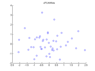
%% Step 3: PCA Whitening
% Complute xPCAWhite and plot the results.
epsilon = 1e-5;
% -------------------- YOUR CODE HERE --------------------
xPCAWhite = zeros(size(x)); % You need to compute this
xPCAWhite = diag(1./sqrt(diag(s)+epsilon))*u'*x; % 每个特征除以对应的特征向量,以使每个特征有一致的方差
% --------------------------------------------------------
figure(4);
scatter(xPCAWhite(1, :), xPCAWhite(2, :));
title('xPCAWhite');
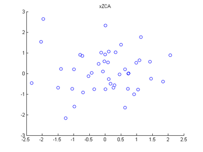
%%================================================================
%% Step 3: ZCA Whitening
% Complute xZCAWhite and plot the results.
% -------------------- YOUR CODE HERE --------------------
xZCAWhite = zeros(size(x)); % You need to compute this
xZCAWhite = u*diag(1./sqrt(diag(s)+epsilon))*u'*x;
% --------------------------------------------------------
figure(5);
scatter(xZCAWhite(1, :), xZCAWhite(2, :));
title('xZCAWhite');
%% Congratulations! When you have reached this point, you are done!
% You can now move onto the next PCA exercise. :)
相关文章推荐
- Stanford UFLDL教程 Exercise:PCA in 2D
- UFLDL——Exercise: PCA in 2D 主成分分析
- UFLDL教程Exercise答案(3.1):PCA in 2D
- Exercise:PCA in 2D 代码示例
- Deep Learning 4_深度学习UFLDL教程:PCA in 2D_Exercise(斯坦福大学深度学习教程)
- 【DeepLearning】Exercise:PCA in 2D
- Convolutional neural networks(CNN) (五) PCA in 2D Exercise
- UFLDL教程答案(3):Exercise:PCA_in_2D&PCA_and_Whitening
- Python数据处理 PCA/ZCA 白化(UFLDL教程:Exercise:PCA_in_2D&PCA_and_Whitening)
- UFLDL教程:Exercise:PCA in 2D & PCA and Whitening
- deep learning之PCA in 2D matlab 实现
- Creating a 2D Active Shape Model in ITK Using PCA
- UFLDL Exercise:PCA in 2D
- UFLDL Exercise:PCA in 2D
- UFLDL Exercise:PCA in 2D
- 2DPCA以及增强的双向2DPCA详解
- 《 Elementary Methods in Number Theory 》Exercise 1.3.12
- 【索引】Geometric Computations in 2D:Exercises: Beginner
- Pixel perfect 2d in 4.3?
- UFLDL教程之(三)PCA and Whitening exercise