Sparse Autoencoder（二）

In this section, we describe a method for numerically checking the derivatives computed by your code to make sure that your implementation is correct. Carrying out the derivative checking procedure described here will significantly increase your confidence in the correctness of your code.

Suppose we want to minimize

as a function of

. For this example, suppose

, so that

. In this 1-dimensional case, one iteration of gradient descent is given by



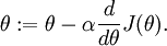
Suppose also that we have implemented some function

that purportedly computes

, so that we implement gradient descent using the update

.

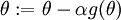
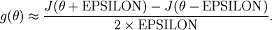
Recall the mathematical definition of the derivative as



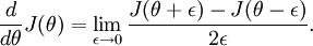
Thus, at any specific value of

, we can numerically approximate the derivative as follows:



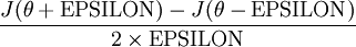
Thus, given a function

that is supposedly computing

, we can now numerically verify its correctness by checking that



The degree to which these two values should approximate each other will depend on the details of

. But assuming

, you'll usually find that the left- and right-hand sides of the above will agree to at least 4 significant digits (and often many more).

Suppose we have a function

that purportedly computes

; we'd like to check if

is outputting correct derivative values. Let

, where



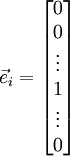
is the

-th basis vector (a vector of the same dimension as

, with a "1" in the

-th position and "0"s everywhere else). So,

is the same as

, except its

-th element has been incremented by EPSILON. Similarly, let

be the corresponding vector with the

-th element decreased by EPSILON. We can now numerically verify

's correctness by checking, for each

, that:



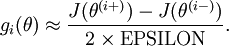
参数为向量，为了验证每一维的计算正确性，可以控制其他变量

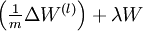
When implementing backpropagation to train a neural network, in a correct implementation we will have that



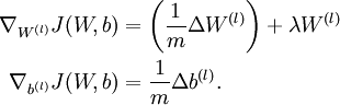
This result shows that the final block of psuedo-code in Backpropagation Algorithm is indeed implementing gradient descent. To make sure your implementation of gradient descent is correct, it is usually very helpful to use the method described above to numerically compute the derivatives of

, and thereby verify that your computations of

and

are indeed giving the derivatives you want.

Anautoencoder neural network is an unsupervised learning algorithm that applies backpropagation, setting the target values to be equal to the inputs. I.e., it uses

.

Here is an autoencoder:





we will write

to denote the activation of this hidden unit when the network is given a specific input

. Further, let



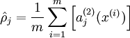
be the average activation of hidden unit

(averaged over the training set). We would like to (approximately) enforce the constraint



where

is a sparsity parameter, typically a small value close to zero (say

). In other words, we would like the average activation of each hidden neuron

to be close to 0.05 (say). To satisfy this constraint, the hidden unit's activations must mostly be near 0.

To achieve this, we will add an extra penalty term to our optimization objective that penalizes

deviating significantly from

. Many choices of the penalty term will give reasonable results. We will choose the following:



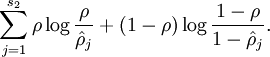
Here,

is the number of neurons in the hidden layer, and the index

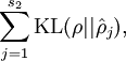
is summing over the hidden units in our network. If you are familiar with the concept of KL divergence, this penalty term is based on it, and can also be written



Our overall cost function is now



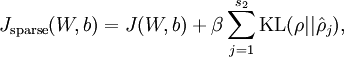
where

is as defined previously, and

controls the weight of the sparsity penalty term. The term

(implicitly) depends on

also, because it is the average activation of hidden unit

, and the activation of a hidden unit depends on the parameters

.

Consider the case of training an autoencoder on

images, so that

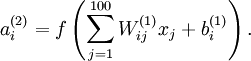
. Each hidden unit

computes a function of the input:



We will visualize the function computed by hidden unit

---which depends on the parameters

(ignoring the bias term for now)---using a 2D image. In particular, we think of

as some non-linear feature of the input


If we suppose that the input is norm constrained by

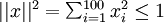
, then one can show (try doing this yourself) that the input which maximally activates hidden unit

is given by setting pixel

(for all 100 pixels,

) to



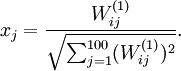
By displaying the image formed by these pixel intensity values, we can begin to understand what feature hidden unit

is looking for.

对一幅图像进行Autoencoder ，前面的隐藏结点一般捕获的是边缘等初级特征，越靠后隐藏结点捕获的特征语义更深。