UFLDL——Exercise: PCA in 2D 主成分分析
2014-12-25 16:24
274 查看
实验要求可以参考deeplearning的tutorial,
Exercise: PCA in 2D。
在实验中,我计算了每一次原始数据,PCA旋转,PCA白化处理,以及ZCA白化处理后的协方差矩阵,结果为:
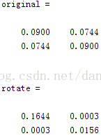
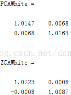
计算协方差我使用了matlab自带的cov(x),它要求矩阵x的每一行代表一个数据,这个tutorial实验说明求得的协方差矩阵的结果不同,为matlab计算的时候需要除以n-1(n为数据的个数),但这些对最后的结果都是没有影响的。
%%================================================================
%% Step 0: Load data
% We have provided the code to load data from pcaData.txt into x.
% x is a 2 * 45 matrix, where the kth column x(:,k) corresponds to
% the kth data point.Here we provide the code to load natural image data into x.
% You do not need to change the code below.
x = load('pcaData.txt','-ascii');
figure(1);
scatter(x(1, :), x(2, :));
title('Raw data');
original = cov(x')%*(size(x,2)-1)
%%================================================================
%% Step 1a: Implement PCA to obtain U
% Implement PCA to obtain the rotation matrix U, which is the eigenbasis
% sigma.
% -------------------- YOUR CODE HERE --------------------
u = zeros(size(x, 1)); % You need to compute this
sigma = x*x'/size(x, 2);
[u,s,v] = svd(sigma);
% --------------------------------------------------------
hold on
plot([0 u(1,1)], [0 u(2,1)]);
plot([0 u(1,2)], [0 u(2,2)]);
scatter(x(1, :), x(2, :));
hold off
%%================================================================
%% Step 1b: Compute xRot, the projection on to the eigenbasis
% Now, compute xRot by projecting the data on to the basis defined
% by U. Visualize the points by performing a scatter plot.
% -------------------- YOUR CODE HERE --------------------
xRot = zeros(size(x)); % You need to compute this
xRot = u'*x;
rotate = cov(xRot')%*(size(x,2)-1)
% --------------------------------------------------------
% Visualise the covariance matrix. You should see a line across the
% diagonal against a blue background.
figure(2);
scatter(xRot(1, :), xRot(2, :));
title('xRot');
%%================================================================
%% Step 2: Reduce the number of dimensions from 2 to 1.
% Compute xRot again (this time projecting to 1 dimension).
% Then, compute xHat by projecting the xRot back onto the original axes
% to see the effect of dimension reduction
% -------------------- YOUR CODE HERE --------------------
k = 1; % Use k = 1 and project the data onto the first eigenbasis
xHat = zeros(size(x)); % You need to compute this
xTiled = zeros(size(x));
xTiled(1:k,:) = xRot(1:k,:);
xHat = u*xTiled;
% --------------------------------------------------------
figure(3);
scatter(xHat(1, :), xHat(2, :));
title('xHat');
%%================================================================
%% Step 3: PCA Whitening
% Complute xPCAWhite and plot the results.
epsilon = 1e-5;
% -------------------- YOUR CODE HERE --------------------
xPCAWhite = zeros(size(x)); % You need to compute this
epsilon = 1e-5;
xPCAWhite = diag(1./sqrt(diag(s) + epsilon)) * xRot;
PCAWhite = cov(xPCAWhite')%*(size(x,2)-1)
% --------------------------------------------------------
figure(4);
scatter(xPCAWhite(1, :), xPCAWhite(2, :));
title('xPCAWhite');
%%================================================================
%% Step 3: ZCA Whitening
% Complute xZCAWhite and plot the results.
% -------------------- YOUR CODE HERE --------------------
xZCAWhite = zeros(size(x)); % You need to compute this
xZCAWhite = u * xPCAWhite;
ZCAWhite = cov(xZCAWhite')%*(size(x,2)-1)
% --------------------------------------------------------
figure(5);
scatter(xZCAWhite(1, :), xZCAWhite(2, :));
title('xZCAWhite');
%% Congratulations! When you have reached this point, you are done!
% You can now move onto the next PCA exercise. :)
Exercise: PCA in 2D。
1. 实验描述:
实验在二维数据上进行PCA降维,PCA白化处理,以及ZCA白化处理,原理可以参考之间的博客,下面直接贴代码。在实验中,我计算了每一次原始数据,PCA旋转,PCA白化处理,以及ZCA白化处理后的协方差矩阵,结果为:
计算协方差我使用了matlab自带的cov(x),它要求矩阵x的每一行代表一个数据,这个tutorial实验说明求得的协方差矩阵的结果不同,为matlab计算的时候需要除以n-1(n为数据的个数),但这些对最后的结果都是没有影响的。
2. 源代码
close all%%================================================================
%% Step 0: Load data
% We have provided the code to load data from pcaData.txt into x.
% x is a 2 * 45 matrix, where the kth column x(:,k) corresponds to
% the kth data point.Here we provide the code to load natural image data into x.
% You do not need to change the code below.
x = load('pcaData.txt','-ascii');
figure(1);
scatter(x(1, :), x(2, :));
title('Raw data');
original = cov(x')%*(size(x,2)-1)
%%================================================================
%% Step 1a: Implement PCA to obtain U
% Implement PCA to obtain the rotation matrix U, which is the eigenbasis
% sigma.
% -------------------- YOUR CODE HERE --------------------
u = zeros(size(x, 1)); % You need to compute this
sigma = x*x'/size(x, 2);
[u,s,v] = svd(sigma);
% --------------------------------------------------------
hold on
plot([0 u(1,1)], [0 u(2,1)]);
plot([0 u(1,2)], [0 u(2,2)]);
scatter(x(1, :), x(2, :));
hold off
%%================================================================
%% Step 1b: Compute xRot, the projection on to the eigenbasis
% Now, compute xRot by projecting the data on to the basis defined
% by U. Visualize the points by performing a scatter plot.
% -------------------- YOUR CODE HERE --------------------
xRot = zeros(size(x)); % You need to compute this
xRot = u'*x;
rotate = cov(xRot')%*(size(x,2)-1)
% --------------------------------------------------------
% Visualise the covariance matrix. You should see a line across the
% diagonal against a blue background.
figure(2);
scatter(xRot(1, :), xRot(2, :));
title('xRot');
%%================================================================
%% Step 2: Reduce the number of dimensions from 2 to 1.
% Compute xRot again (this time projecting to 1 dimension).
% Then, compute xHat by projecting the xRot back onto the original axes
% to see the effect of dimension reduction
% -------------------- YOUR CODE HERE --------------------
k = 1; % Use k = 1 and project the data onto the first eigenbasis
xHat = zeros(size(x)); % You need to compute this
xTiled = zeros(size(x));
xTiled(1:k,:) = xRot(1:k,:);
xHat = u*xTiled;
% --------------------------------------------------------
figure(3);
scatter(xHat(1, :), xHat(2, :));
title('xHat');
%%================================================================
%% Step 3: PCA Whitening
% Complute xPCAWhite and plot the results.
epsilon = 1e-5;
% -------------------- YOUR CODE HERE --------------------
xPCAWhite = zeros(size(x)); % You need to compute this
epsilon = 1e-5;
xPCAWhite = diag(1./sqrt(diag(s) + epsilon)) * xRot;
PCAWhite = cov(xPCAWhite')%*(size(x,2)-1)
% --------------------------------------------------------
figure(4);
scatter(xPCAWhite(1, :), xPCAWhite(2, :));
title('xPCAWhite');
%%================================================================
%% Step 3: ZCA Whitening
% Complute xZCAWhite and plot the results.
% -------------------- YOUR CODE HERE --------------------
xZCAWhite = zeros(size(x)); % You need to compute this
xZCAWhite = u * xPCAWhite;
ZCAWhite = cov(xZCAWhite')%*(size(x,2)-1)
% --------------------------------------------------------
figure(5);
scatter(xZCAWhite(1, :), xZCAWhite(2, :));
title('xZCAWhite');
%% Congratulations! When you have reached this point, you are done!
% You can now move onto the next PCA exercise. :)

相关文章推荐
- UFLDL教程答案(3):Exercise:PCA_in_2D&PCA_and_Whitening
- Deep Learning 4_深度学习UFLDL教程:PCA in 2D_Exercise(斯坦福大学深度学习教程)
- UFLDL教程Exercise答案(3.1):PCA in 2D
- UFLDL教程:Exercise:PCA in 2D & PCA and Whitening
- Python数据处理 PCA/ZCA 白化(UFLDL教程:Exercise:PCA_in_2D&PCA_and_Whitening)
- 深度学习入门教程UFLDL学习实验笔记三:主成分分析PCA与白化whitening
- Convolutional neural networks(CNN) (五) PCA in 2D Exercise
- 深度学习入门教程UFLDL学习实验笔记三:主成分分析PCA与白化whitening
- Stanford UFLDL教程 Exercise:PCA in 2D
- Loadings vs eigenvectors in PCA 主成分分析(PCA)中的负荷和特征向量
- Exercise:PCA in 2D 代码示例
- 【DeepLearning】Exercise:PCA in 2D
- Exercise: PCA in 2D
- 机器学习中的数学(4)-线性判别分析(LDA), 主成分分析(PCA)
- 线性判别分析(LDA), 主成分分析(PCA)
- PCA--主成分分析
- 线性判别分析(LDA), 主成分分析(PCA)
- 机器学习中的数学(4)-线性判别分析(LDA), 主成分分析(PCA)
- 机器学习中的数学(4)-线性判别分析(LDA), 主成分分析(PCA)
- 主成分分析PCA