Sparse Autoencoder3-Gradient checking and advanced optimization

原文：http://deeplearning.stanford.edu/wiki/index.php/Gradient_checking_and_advanced_optimization

Backpropagation is a notoriously difficult algorithm to debug and get right, especially since many subtly buggy implementations of it—for example, one that has an off-by-one error in the indices and that thus only trains some of the layers of weights, or an
implementation that omits the bias term—will manage to learn something that can look surprisingly reasonable (while performing less well than a correct implementation). Thus, even with a buggy implementation, it may not at all be apparent that anything is
amiss. In this section, we describe a method for numerically checking the derivatives computed by your code to make sure that your implementation is correct. Carrying out the derivative checking procedure described here will significantly increase your confidence
in the correctn
4000
ess of your code.

Suppose we want to minimize 

 as a function of 

.
For this example, suppose 

, so that 

.
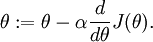
In this 1-dimensional case, one iteration of gradient descent is given by



Suppose also that we have implemented some function 

 that purportedly
computes 

, so that we implement gradient
descent using the update 

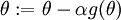
. How can
we check if our implementation of 

 is correct?

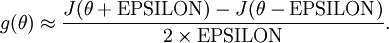
Recall the mathematical definition of the derivative as



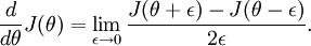
Thus, at any specific value of 

, we can numerically approximate
the derivative as follows:



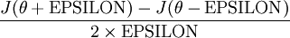
In practice, we set EPSILON to a small constant, say around 

.
(There's a large range of values of EPSILON that should work well, but we don't set EPSILON to be "extremely" small, say 

,
as that would lead to numerical roundoff errors.)

Thus, given a function 

 that is supposedly computing 

,
we can now numerically verify its correctness by checking that



The degree to which these two values should approximate each other will depend on the details of 

.
But assuming 

, you'll usually find that the
left- and right-hand sides of the above will agree to at least 4 significant digits (and often many more).

Now, consider the case where 

 is a vector rather than
a single real number (so that we have 

 parameters that we want to
learn), and 

. In our neural network example we
used "

," but one can imagine "unrolling" the parameters 

 into
a long vector 

. We now generalize our derivative checking procedure
to the case where 

 may be a vector.

Suppose we have a function 

 that purportedly computes 

;
we'd like to check if 

 is outputting correct derivative values.
Let 

, where



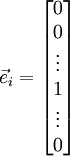
is the 

-th basis vector (a vector of the same dimension as 

,
with a "1" in the 

-th position and "0"s everywhere else). So, 

 is
the same as 

, except its 

-th
element has been incremented by EPSILON. Similarly, let 

be
the corresponding vector with the 

-th element decreased by EPSILON.
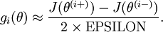
We can now numerically verify 

's correctness by checking,
for each 

, that:



When implementing backpropagation to train a neural network, in a correct implementation we will have that



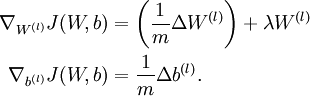
This result shows that the final block of psuedo-code in Backpropagation Algorithm is
indeed implementing gradient descent. To make sure your implementation of gradient descent is correct, it is usually very helpful to use the method described above to numerically compute the derivatives of 

,
and thereby verify that your computations of 

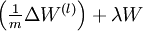
 and 

 are
indeed giving the derivatives you want.

Finally, so far our discussion has centered on using gradient descent to minimize 

.
If you have implemented a function that computes 

 and 

,
it turns out there are more sophisticated algorithms than gradient descent for trying to minimize 

.
For example, one can envision an algorithm that uses gradient descent, but automatically tunes the learning rate 

 so
as to try to use a step-size that causes 

 to approach a local
optimum as quickly as possible. There are other algorithms that are even more sophisticated than this; for example, there are algorithms that try to find an approximation to the Hessian matrix, so that it can take more rapid steps towards a local optimum (similar
to Newton's method). A full discussion of these algorithms is beyond the scope of these notes, but one example is the L-BFGS algorithm. (Another example is the conjugate gradient algorithm.) You will use one of these algorithms
in the programming exercise. The main thing you need to provide to these advanced optimization algorithms is that for any 

,
you have to be able to compute 

and 

.
These optimization algorithms will then do their own internal tuning of the learning rate/step-size 

 (and
compute its own approximation to the Hessian, etc.) to automatically search for a value of 

 that
minimizes 

. Algorithms such as L-BFGS and conjugate gradient
can often be much faster than gradient descent.