Sparse Autoencoder1-NeuralNetworks
2013-03-25 17:21
495 查看
原文:http://deeplearning.stanford.edu/wiki/index.php/Neural_Networks
Consider a supervised learning problem where we have access to labeled training examples (x(i),y(i)). Neural networks give a way of defining a complex,
non-linear form of hypotheses hW,b(x), with parameters W,b that we can fit to our
data.
To describe neural networks, we will begin by describing the simplest possible neural network, one which comprises a single "neuron." We will use the following diagram to denote a single neuron:
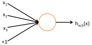
This "neuron" is a computational unit that takes as input x1,x2,x3 (and a +1 intercept term), and outputs

,
where

is called the activation function.
In these notes, we will choose

to be the sigmoid function:
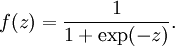
Thus, our single neuron corresponds exactly to the input-output mapping defined by logistic regression.
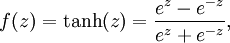
Although these notes will use the sigmoid function, it is worth noting that another common choice for f is the hyperbolic tangent, or tanh, function:
Here are plots of the sigmoid and tanh functions:
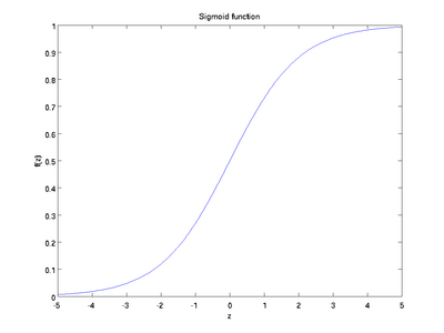
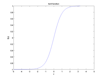
The tanh(z) function is a rescaled version of the sigmoid, and its output range is [ − 1,1] instead of [0,1].
Note that unlike some other venues (including the OpenClassroom videos, and parts of CS229), we are not using the convention here of x0 = 1. Instead, the intercept term is handled separately
by the parameter b.
Finally, one identity that'll be useful later: If f(z) = 1 / (1 + exp( − z)) is the sigmoid function, then its derivative is given by f'(z)
= f(z)(1 − f(z)). (If f is the tanh function, then its derivative is given by f'(z)
= 1 − (f(z))2.) You can derive this yourself using the definition of the sigmoid (or tanh) function.
A neural network is put together by hooking together many of our simple "neurons," so that the output of a neuron can be the input of another. For example, here is a small neural network:
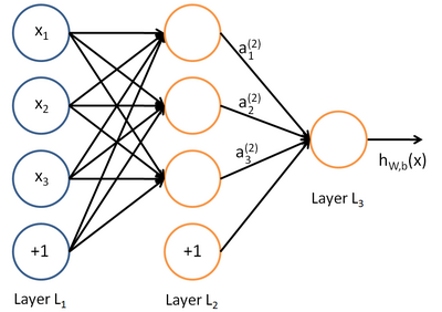
In this figure, we have used circles to also denote the inputs to the network. The circles labeled "+1" are called bias units, and correspond to the intercept term. The leftmost layer of the network is called the input layer,
and the rightmost layer the output layer (which, in this example, has only one node). The middle layer of nodes is called thehidden layer, because its values are not observed in the training set. We also say that our example
neural network has 3input units (not counting the bias unit), 3 hidden units, and 1 output unit.
We will let nl denote the number of layers in our network; thus nl = 3 in our example. We
label layer l as Ll, so layer L1is
the input layer, and layer

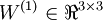
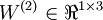
the output layer. Our neural network has parameters (W,b)
= (W(1),b(1),W(2),b(2)), where we write

to
denote the parameter (or weight) associated with the connection between unit j in layer l, and unit i in
layer l + 1. (Note the order of the indices.) Also,

is
the bias associated with unit i in layer l + 1. Thus, in our example, we have
,
and
. Note that bias units don't have inputs or connections
going into them, since they always output the value +1. We also let sl denote the number of nodes in layer l (not
counting the bias unit).
We will write

to denote the activation (meaning output
value) of unit i in layer l. For l = 1, we also use

to
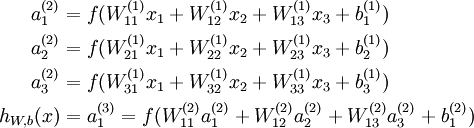
denote the i-th input. Given a fixed setting of the parameters W,b, our neural network defines a hypothesis hW,b(x) that
outputs a real number. Specifically, the computation that this neural network represents is given by:
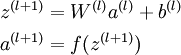
In the sequel, we also let

denote the total weighted sum of inputs to
unit i in layer l, including the bias term (e.g.,
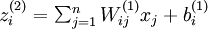
),
so that
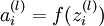
.
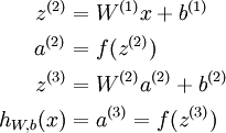
Note that this easily lends itself to a more compact notation. Specifically, if we extend the activation function
to
apply to vectors in an element-wise fashion (i.e., f([z1,z2,z3]) = [f(z1),f(z2),f(z3)]),
then we can write the equations above more compactly as:
We call this step forward propagation. More generally, recalling that we also use a(1) = x to also denote the values from the input layer, then given layer l's
activations a(l), we can compute layer l + 1's activations a(l +
1) as:
By organizing our parameters in matrices and using matrix-vector operations, we can take advantage of fast linear algebra routines to quickly perform calculations in our network.
We have so far focused on one example neural network, but one can also build neural networks with other architectures(meaning patterns of connectivity between neurons), including ones with multiple hidden layers. The most common choice is a

-layered
network where layer

is the input layer, layer
is
the output layer, and each layer

is densely connected to layer

.
In this setting, to compute the output of the network, we can successively compute all the activations in layer

,
then layer

, and so on, up to layer

,
using the equations above that describe the forward propagation step. This is one example of a feedforward neural network, since the connectivity graph does not have any directed loops or cycles.
Neural networks can also have multiple output units. For example, here is a network with two hidden layers layers L2 and L3and
two output units in layer L4:
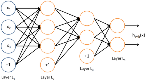
To train this network, we would need training examples (x(i),y(i)) where

.
This sort of network is useful if there're multiple outputs that you're interested in predicting. (For example, in a medical diagnosis application, the vector x might give the input features of
a patient, and the different outputs yi's might indicate presence or absence of different diseases.)
Consider a supervised learning problem where we have access to labeled training examples (x(i),y(i)). Neural networks give a way of defining a complex,
non-linear form of hypotheses hW,b(x), with parameters W,b that we can fit to our
data.
To describe neural networks, we will begin by describing the simplest possible neural network, one which comprises a single "neuron." We will use the following diagram to denote a single neuron:

This "neuron" is a computational unit that takes as input x1,x2,x3 (and a +1 intercept term), and outputs
,
where
is called the activation function.
In these notes, we will choose
to be the sigmoid function:
Thus, our single neuron corresponds exactly to the input-output mapping defined by logistic regression.
Although these notes will use the sigmoid function, it is worth noting that another common choice for f is the hyperbolic tangent, or tanh, function:
Here are plots of the sigmoid and tanh functions:


The tanh(z) function is a rescaled version of the sigmoid, and its output range is [ − 1,1] instead of [0,1].
Note that unlike some other venues (including the OpenClassroom videos, and parts of CS229), we are not using the convention here of x0 = 1. Instead, the intercept term is handled separately
by the parameter b.
Finally, one identity that'll be useful later: If f(z) = 1 / (1 + exp( − z)) is the sigmoid function, then its derivative is given by f'(z)
= f(z)(1 − f(z)). (If f is the tanh function, then its derivative is given by f'(z)
= 1 − (f(z))2.) You can derive this yourself using the definition of the sigmoid (or tanh) function.
Neural Network model
A neural network is put together by hooking together many of our simple "neurons," so that the output of a neuron can be the input of another. For example, here is a small neural network:
In this figure, we have used circles to also denote the inputs to the network. The circles labeled "+1" are called bias units, and correspond to the intercept term. The leftmost layer of the network is called the input layer,
and the rightmost layer the output layer (which, in this example, has only one node). The middle layer of nodes is called thehidden layer, because its values are not observed in the training set. We also say that our example
neural network has 3input units (not counting the bias unit), 3 hidden units, and 1 output unit.
We will let nl denote the number of layers in our network; thus nl = 3 in our example. We
label layer l as Ll, so layer L1is
the input layer, and layer
the output layer. Our neural network has parameters (W,b)
= (W(1),b(1),W(2),b(2)), where we write
to
denote the parameter (or weight) associated with the connection between unit j in layer l, and unit i in
layer l + 1. (Note the order of the indices.) Also,
is
the bias associated with unit i in layer l + 1. Thus, in our example, we have
,
and
. Note that bias units don't have inputs or connections
going into them, since they always output the value +1. We also let sl denote the number of nodes in layer l (not
counting the bias unit).
We will write
to denote the activation (meaning output
value) of unit i in layer l. For l = 1, we also use
to
denote the i-th input. Given a fixed setting of the parameters W,b, our neural network defines a hypothesis hW,b(x) that
outputs a real number. Specifically, the computation that this neural network represents is given by:
In the sequel, we also let
denote the total weighted sum of inputs to
unit i in layer l, including the bias term (e.g.,
),
so that
.
Note that this easily lends itself to a more compact notation. Specifically, if we extend the activation function
to
apply to vectors in an element-wise fashion (i.e., f([z1,z2,z3]) = [f(z1),f(z2),f(z3)]),
then we can write the equations above more compactly as:
We call this step forward propagation. More generally, recalling that we also use a(1) = x to also denote the values from the input layer, then given layer l's
activations a(l), we can compute layer l + 1's activations a(l +
1) as:
By organizing our parameters in matrices and using matrix-vector operations, we can take advantage of fast linear algebra routines to quickly perform calculations in our network.
We have so far focused on one example neural network, but one can also build neural networks with other architectures(meaning patterns of connectivity between neurons), including ones with multiple hidden layers. The most common choice is a
-layered
network where layer
is the input layer, layer
is
the output layer, and each layer
is densely connected to layer
.
In this setting, to compute the output of the network, we can successively compute all the activations in layer
,
then layer
, and so on, up to layer
,
using the equations above that describe the forward propagation step. This is one example of a feedforward neural network, since the connectivity graph does not have any directed loops or cycles.
Neural networks can also have multiple output units. For example, here is a network with two hidden layers layers L2 and L3and
two output units in layer L4:

To train this network, we would need training examples (x(i),y(i)) where
.
This sort of network is useful if there're multiple outputs that you're interested in predicting. (For example, in a medical diagnosis application, the vector x might give the input features of
a patient, and the different outputs yi's might indicate presence or absence of different diseases.)

相关文章推荐
- Sparse Bundle Adhustment 1.5使用指南
- matlab sparse
- sparse bayesian model
- RMQ问题之Sparse_Table算法
- 稀疏表达:向量、矩阵与张量(上)(转载自http://www.cvchina.info/2010/06/01/sparse-representation-vector-matrix-tensor-1)
- scipy.sparse求稀疏矩阵前k个特征值
- Sparse Autoencoder2-Backpropagation Algorithm
- 稀疏数组(Sparse array)
- Deep Learning论文笔记之(二)Sparse Filtering稀疏滤波
- 《Sparse and Redundant Representations》第二章:唯一性与不确定性
- RMQ (Range Minimum/Maximum Query)问题的ST(Sparse Table)解法
- 《Gabor feature based sparse representation for face recognition with gabor occlusion dictionary》
- Sparse Feature Learning
- PIM Sparse-Mode 中 RP 的三种定义方法(static、AutoRP、BSR)
- 内核工具 – Sparse 简介
- Sparse Filtering 学习笔记(三)目标函数的建立和求解
- Deep Learning模型之:Sparse Coding
- sparse bundle adju 997b stment(sba) 摄影测量光束法平差程序库------程序库简介
- Sparse coding
- Eigen sparse 基本操作:构造 & 输出