Sparse Autoencoder2-Backpropagation Algorithm

原文：http://deeplearning.stanford.edu/wiki/index.php/Backpropagation_Algorithm

Suppose we have a fixed training set 

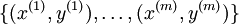
 of m training
examples. We can train our neural network using batch gradient descent. In detail, for a single training example (x,y), we define the cost function with respect to that single example
to be:



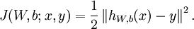
This is a (one-half) squared-error cost function. Given a training set of m examples, we then define the overall cost function to be:



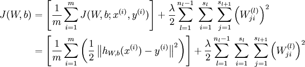
The first term in the definition of J(W,b) is an average sum-of-squares error term. The second term is a regularization term (also called a weight decay term)
that tends to decrease the magnitude of the weights, and helps prevent overfitting.

[Note: Usually weight decay is not applied to the bias terms 

, as reflected
in our definition for J(W,b). Applying weight decay to the bias units usually makes only a small difference to the final network, however. If you've taken CS229 (Machine Learning)
at Stanford or watched the course's videos on YouTube, you may also recognize this weight decay as essentially a variant of the Bayesian regularization method you saw there, where we placed a Gaussian prior on the parameters and did MAP (instead of maximum
likelihood) estimation.]

The weight decay parameter λ controls the relative importance of the two terms. Note also the slightly overloaded notation: J(W,b;x,y) is
the squared error cost with respect to a single example; J(W,b) is the overall cost function, which includes the weight decay term.

This cost function above is often used both for classification and for regression problems. For classification, we let y = 0 or 1 represent
the two class labels (recall that the sigmoid activation function outputs values in [0,1]; if we were using a tanh activation function, we would instead use -1 and +1 to denote the labels). For regression
problems, we first scale our outputs to ensure that they lie in the [0,1] range (or if we were using a tanh activation function, then the [ − 1,1] range).

Our goal is to minimize J(W,b) as a function of W and b.
To train our neural network, we will initialize each parameter 

 and
each 

 to a small random value near zero (say according to a Normal(0,ε2) distribution
for some small ε, say0.01), and then apply an optimization algorithm such as batch gradient descent. Since J(W,b) is
a non-convex function, gradient descent is susceptible to local optima; however, in practice gradient descent usually works fairly well. Finally, note that it is important to initialize the parameters randomly, rather than to all 0's. If all the parameters
start off at identical values, then all the hidden layer units will end up learning the same function of the input (more formally, 

will
be the same for all values of i, so that 

 for
any input x). The random initialization serves the purpose of symmetry breaking.

One iteration of gradient descent updates the parameters W,b as follows:



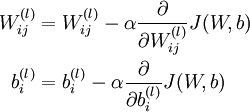
where α is the learning rate. The key step is computing the partial derivatives above. We will now describe thebackpropagation algorithm, which gives an efficient way to compute these partial
derivatives.

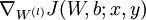
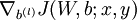
We will first describe how backpropagation can be used to compute 

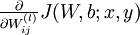
 and 

,
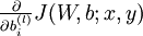
the partial derivatives of the cost function J(W,b;x,y) defined with respect to a single example (x,y).
Once we can compute these, we see that the derivative of the overall cost function <
d9b4
em>J(W,b) can be computed as:



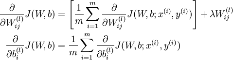
The two lines above differ slightly because weight decay is applied to W but not b.

The intuition behind the backpropagation algorithm is as follows. Given a training example (x,y), we will first run a "forward pass" to compute all the activations throughout the network,
including the output value of the hypothesis hW,b(x). Then, for each node i in layer l,
we would like to compute an "error term" 

 that measures how much
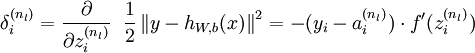
that node was "responsible" for any errors in our output. For an output node, we can directly measure the difference between the network's activation and the true target value, and use that to define 

 (where
layer nl is the output layer). How about hidden units? For those, we will compute 

 based
on a weighted average of the error terms of the nodes that uses 

 as an
input. In detail, here is the backpropagation algorithm:
Perform a feedforward pass, computing the activations for layers L2, L3, and
so on up to the output layer 

.
For each output unit i in layer nl (the output layer), set



For 


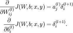
For each node i in layer l, set



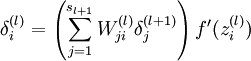
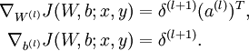
Compute the desired partial derivatives, which are given as:



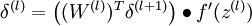
Finally, we can also re-write the algorithm using matrix-vectorial notation. We will use "

"
to denote the element-wise product operator (denoted ".*" in Matlab or Octave, and also called the Hadamard product), so that if 

,
then 

. Similar to how we extended the definition of 

 to
apply element-wise to vectors, we also do the same for 

(so
that 

).

The algorithm can then be written:
Perform a feedforward pass, computing the activations for layers 

, 

,
up to the output layer 

, using the equations defining the forward propagation
steps
For the output layer (layer 

), set



For 


Set



Compute the desired partial derivatives:



Implementation note: In steps 2 and 3 above, we need to compute 

 for
each value of 

. Assuming 

 is
the sigmoid activation function, we would already have 

 stored
away from the forward pass through the network. Thus, using the expression that we worked out earlier for 

,
we can compute this as 

.

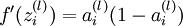
Finally, we are ready to describe the full gradient descent algorithm. In the pseudo-code below, 

 is
a matrix (of the same dimension as 

), and 

 is
a vector (of the same dimension as 

). Note that in this notation,
"

" is a matrix, and in particular it isn't "

 times 

."
We implement one iteration of batch gradient descent as follows:
Set 

, 

 (matrix/vector
of zeros) for all 

.
For 

 to 

,
Use backpropagation to compute 

 and 

.
Set 

.
Set 

.

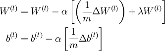
Update the parameters:



To train our neural network, we can now repeatedly take steps of gradient descent to reduce our cost function 

.