线性回归的N种姿势

1. Naive Solution

We want to find x̂ x^ that minimizes:

∣∣∣∣Ax̂ −b∣∣∣∣2||Ax^−b||2

Another way to think about this is that we are interested in where vector bb​ is closest to the subspace spanned by AA​ (called the range of AA​). Ax̂ Ax^​ is the projection of bb​ onto AA​. Since b−Ax̂ b−Ax^​ must be perpendicular to the subspace spanned by AA​, we see that

AT(b−Ax̂ )=0AT(b−Ax^)=0



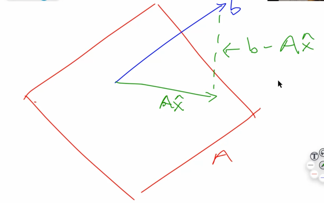
(we are using ATAT because we want to multiply each column of AA by b−Ax̂ b−Ax^

This leads us to the normal equations:

x=(ATA)−1ATbx=(ATA)−1ATb

但是这种方法不是很practical，因为要求矩阵的逆，比较麻烦。

def ls_naive(A, b):
# not practical，因为直接求了矩阵的逆，很麻烦
return np.linalg.inv(A.T @ A) @ A.T @ b

coeffs_naive = ls_naive(trn_int, y_trn)
regr_metrics(y_test, test_int @ coeffs_naive)

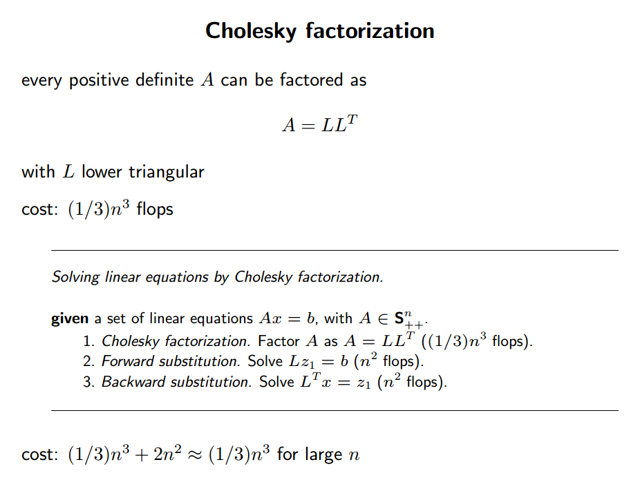
2. Cholesky Factorization

Normal equations:

ATAx=ATbATAx=ATb

If AA has full rank, the pseudo-inverse (ATA)−1AT(ATA)−1AT is a square, hermitian positive definite matrix.

【注意】Cholesky一定要是正定矩阵！虽然这个操作又快又好，但是使用场景有限！

The standard way of solving such a system is Cholesky Factorization, which finds upper-triangular R such that ATA=RTRATA=RTR. ( RTRT is lower-triangular )

AtA = A.T @ A
Atb = A.T @ b

R = scipy.linalg.cholesky(AtA)

# check our factorization
np.linalg.norm(AtA - R.T @ R)

Q：为啥变成 RTRx=ATbRTRx=ATb 会变简单？

之前提过，上三角矩阵解线性方程组时会简单许多（最后一行只有一个未知数）。

所以先求 RTw=ATbRTw=ATb 再求 Rx=wRx=w 会easier。

ATAx=ATbRTRx=ATbRTw=ATbRx=wATAx=ATbRTRx=ATbRTw=ATbRx=w

def ls_chol(A, b):
R = scipy.linalg.cholesky(A.T @ A)
w = scipy.linalg.solve_triangular(R, A.T @ b, trans='T')
return scipy.linalg.solve_triangular(R, w)

%timeit coeffs_chol = ls_chol(trn_int, y_trn)

3. QR Factorization

QQ is orthonormal, RR is upper-triangular.

Ax=bA=QRQRx=bQ−1=QTQTQRx=QTbRx=QTbAx=bA=QRQRx=bQ−1=QTQTQRx=QTbRx=QTb

Then once again, RxRx is easier to solve than AxAx.

def ls_qr(A,b):
Q, R = scipy.linalg.qr(A, mode='economic')
return scipy.linalg.solve_triangular(R, Q.T @ b)

coeffs_qr = ls_qr(trn_int, y_trn)
regr_metrics(y_test, test_int @ coeffs_qr)

4. SVD

都是同样的问题，要求 xx。 UU 的column orthonormal，∑∑ 是对角阵，VV 是row orthonormal.

Ax=bA=UΣVΣVx=UTbΣw=UTbx=VTwAx=bA=UΣVΣVx=UTbΣw=UTbx=VTw

解 Σw=UTbΣw=UTb 甚至比上三角矩阵 RR 更简单（每行只有一个未知量）。然后 Vx=wVx=w 又可以直接用orthonormal的性质，直接等于 VTwVTw。

SVD gives the pseudo-inverse.

def ls_svd(A,b):
m, n = A.shape
U, sigma, Vh = scipy.linalg.svd(A, full_matrices=False, lapack_driver='gesdd')
w = (U.T @ b)/ sigma
return Vh.T @ w

coeffs_svd = ls_svd(trn_int, y_trn)
regr_metrics(y_test, test_int @ coeffs_svd)

5. Timing Comparison

Matrix Inversion: 2n32n3

Matrix Multiplication: n3n3

Cholesky: 13n313n3

QR, Gram Schmidt: 2mn22mn2, m≥nm≥n (chapter 8 of Trefethen)

QR, Householder: 2mn2−23n32mn2−23n3 (chapter 10 of Trefethen)

Solving a triangular system: n2n2



Why Cholesky Factorization is Fast:



(source: Stanford Convex Optimization: Numerical Linear Algebra Background Slides)