深度学习你不可不知的技巧

转自 https://zhuanlan.zhihu.com/p/21952042

Deep Neural Networks, especially Convolutional Neural Networks (CNN), allows computational
models that are composed of multiple processing layers to learn representations of data with multiple levels of abstraction. These methods have dramatically improved the state-of-the-arts in visual object recognition, object detection, text recognition and
many other domains such as drug discovery and genomics.

In addition, many solid papers have been published in this topic, and some high quality open source CNN software packages have been made available. There are also well-written CNN tutorials or CNN software manuals.
However, it might lack a recent and comprehensive summary about the details of how to implement an excellent deep convolutional neural networks from scratch. Thus, we collected and concluded many implementation details for DCNNs. Here
we will introduce these extensive implementation details, i.e., tricks or tips, for building and training your own deep networks.
Introduction

We assume you already know the basic knowledge of deep learning, and here we will present the implementation details (tricks or tips) in Deep Neural Networks, especially CNN for image-related tasks, mainly in eight
aspects: 1) data augmentation; 2) pre-processing on images; 3) initializations of Networks; 4) some tips during training; 5) selections of activation functions; 6) diverse regularizations; 7)some insights
found from figures and finally 8) methods of ensemble multiple deep networks.
Additionally, the corresponding slides are available at [slide]（http://lamda.nju.edu.cn/weixs/slide/CNNTricks_slide.pdf）.
If there are any problems/mistakes in these materials and slides, or there are something important/interesting you consider that should be added, just feel free to contact me（http://lamda.nju.edu.cn/weixs/?AspxAutoDetectCookieSupport=1）.
Sec. 1: Data Augmentation

Since deep networks need to be trained on a huge number of training images to achieve satisfactory performance, if the original image data set contains limited training images, it is better to do data augmentation
to boost the performance. Also, data augmentation becomes the thing must to do when training a deep network.

1.There are many ways to do data augmentation, such as the popular horizontally flipping, random crops and color jittering. Moreover, you could try combinations of multiple different processing, e.g., doing
the rotation and random scaling at the same time. In addition, you can try to raise saturation and value (S and V components of the HSV color space) of all pixels to a power between 0.25 and 4 (same for all pixels within a patch), multiply these values by
a factor between 0.7 and 1.4, and add to them a value between -0.1 and 0.1. Also, you could add a value between [-0.1, 0.1] to the hue (H component of HSV) of all pixels in the image/patch.
2.Krizhevsky et al. [1] proposed fancy PCA when training the famous Alex-Net in 2012. Fancy PCA alters the intensities of the RGB channels in training images. In practice, you can firstly perform PCA on the
set of RGB pixel values throughout your training images. And then, for each training image, just add the following quantity to each RGB image pixel (i.e.,

):

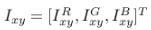
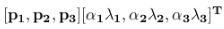
where
, pi and

are
the i-th eigenvector and eigenvalue of the 3*3 covariance matrix of RGB pixel values, respectively, and ai is a random variable drawn from a Gaussian with mean zero and standard deviation 0.1. Please note that, each ai is drawn only once for all the pixels
of a particular training image until that image is used for training again. That is to say, when the model meets the same training image again, it will randomly produce another ai for data augmentation. In [1], they claimed that “fancy PCA could approximately
capture an important property of natural images, namely, that object identity is invariant to changes in the intensity and color of the illumination”. To the classification performance, this scheme reduced the top-1 error rate by over 1% in the competition
of ImageNet 2012.

Sec. 2: Pre-Processing

Now we have obtained a large number of training samples (images/crops), but please do not hurry! Actually, it is necessary to do pre-processing on these images/crops. In this section, we will introduce several
approaches for pre-processing.
The first and simple pre-processing approach is zero-center the data, and then normalize them, which is presented as two lines Python codes as follows:

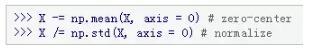
where,
X is the input data (NumIns×NumDim). Another form of this pre-processing normalizes each dimension so that the min and max along the dimension is -1 and 1 respectively. It only makes sense to apply this pre-processing if you have a reason to believe that different
input features have different scales (or units), but they should be of approximately equal importance to the learning algorithm. In case of images, the relative scales of pixels are already approximately equal (and in range from 0 to 255), so it is not strictly
necessary to perform this additional pre-processing step.

Another pre-processing approach similar to the first one is PCA Whitening. In this process, the data is first centered as described above. Then, you can compute the covariance matrix that tells us about the
correlation structure in the data:

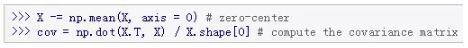
After
that, you decorrelate the data by projecting the original (but zero-centered) data into the eigenbasis:

The
last transformation is whitening, which takes the data in the eigenbasis and divides every dimension by the eigenvalue to normalize the scale:

Note
that here it adds 1e-5 (or a small constant) to prevent division by zero. One weakness of this transformation is that it can greatly exaggerate the noise in the data, since it stretches all dimensions (including the irrelevant dimensions of tiny variance that
are mostly noise) to be of equal size in the input. This can in practice be mitigated by stronger smoothing (i.e., increasing 1e-5 to be a larger number).
Please note that, we describe these pre-processing here just for completeness. In practice, these transformations are not used with Convolutional Neural Networks. However, it is also very important to zero-center
the data, and it is common to see normalization of every pixel as well.
Sec. 3: Initializations

Now the data is ready. However, before you are beginning to train the network, you have to initialize its parameters.1.All Zero Initialization
In the ideal situation, with proper data normalization it is reasonable to assume that approximately half of the weights will be positive and half of them will be negative. A reasonable-sounding idea then might
be to set all the initial weights to zero, which you expect to be the “best guess” in expectation. But, this turns out to be a mistake, because if every neuron in the network computes the same output, then they will also all compute the same gradients during
back-propagation and undergo the exact same parameter updates. In other words, there is no source of asymmetry between neurons if their weights are initialized to be the same.

2.Initialization with Small Random Numbers
Thus, you still want the weights to be very close to zero, but not identically zero. In this way, you can random these neurons to small numbers which are very close to zero, and it is treated as symmetry breaking.
The idea is that the neurons are all random and unique in the beginning, so they will compute distinct updates and integrate themselves as diverse parts of the full network. The implementation for weights might simply look like

,
where

is
a zero mean, unit standard deviation gaussian. It is also possible to use small numbers drawn from a uniform distribution, but this seems to have relatively little impact on the final performance in practice.

3.Calibrating the Variances One problem with the above suggestion is that the distribution of the outputs from a randomly initialized
neuron has a variance that grows with the number of inputs. It turns out that you can normalize the variance of each neuron's output to 1 by scaling its weight vector by the square root of its fan-in (i.e., its number of inputs), which is as follows:

where
“randn” is the aforementioned Gaussian and “n” is the number of its inputs. This ensures that all neurons in the network initially have approximately the same output distribution and empirically improves the rate of convergence. The detailed derivations can
be found from Page. 18 to 23 of the slides. Please note that, in the derivations, it does not consider the influence of ReLU neurons.

4.Current Recommendation
As aforementioned, the previous initialization by calibrating the variances of neurons is without considering ReLUs. A more recent paper on this topic by He et al. [4] derives an initialization specifically
for ReLUs, reaching the conclusion that the variance of neurons in the network should be 2.0/n as:


Sec. 4: During Training

Now, everything is ready. Let’s start to train deep networks!

Filters and pooling size. During training, the size of input images prefers to be power-of-2, such as 32 (e.g., CIFAR-10), 64, 224 (e.g.,
common used ImageNet), 384 or 512, etc. Moreover, it is important to employ a small filter (e.g., 3*3 ) and small strides (e.g., 1) with zeros-padding, which not only reduces the number of parameters, but improves the accuracy rates of the whole deep network.
Meanwhile, a special case mentioned above, i.e., 3*3 filters with stride 1, could preserve the spatial size of images/feature maps. For the pooling layers, the common used pooling size is of 2*2. Learning
rate.In addition, as described in a blog by Ilya Sutskever [2], he recommended to divide the gradients by mini batch size. Thus, you should not always change the learning rates (LR), if you change the
mini batch size. For obtaining an appropriate LR, utilizing the validation set is an effective way. Usually, a typical value of LR in the beginning of your training is 0.1. In practice, if you see that you stopped making progress on the validation set, divide
the LR by 2 (or by 5), and keep going, which might give you a surprise.
Fine-tune on pre-trained models. Nowadays, many state-of-the-arts deep networks are released by famous research groups, i.e.,Caffe Model
Zoo(https://github.com/BVLC/caffe/wiki/Model-Zoo)
and VGG Group(http://www.vlfeat.org/matconvnet/pretrained/).
Thanks to the wonderful generalization abilities of pre-trained deep models, you could employ these pre-trained models for your own applications directly. For further improving the classification performance on your data set, a very simple yet effective approach
is to fine-tune the pre-trained models on your own data. As shown in following table, the two most important factors are the size of the new data set (small or big), and its similarity to the original data set. Different strategies of fine-tuning can be utilized
in different situations. For instance, a good case is that your new data set is very similar to the data used for training pre-trained models. In that case, if you have very little data, you can just train a linear classifier on the features extracted from
the top layers of pre-trained models. If your have quite a lot of data at hand, please fine-tune a few top layers of pre-trained models with a small learning rate. However, if your own data set is quite different from the data used in pre-trained models but
with enough training images, a large number of layers should be fine-tuned on your data also with a small learning rate for improving performance. However, if your data set not only contains little data, but is very different from the data used in pre-trained
models, you will be in trouble. Since the data is limited, it seems better to only train a linear classifier. Since the data set is very different, it might not be best to train the classifier from the top of the network, which contains more dataset-specific
features. Instead, it might work better to train the SVM classifier on activations/features from somewhere earlier in the network.

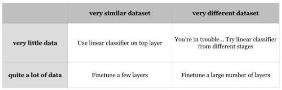
Fine-tune
your data on pre-trained models. Different strategies of fine-tuning are utilized in different situations. For data sets, Caltech-101 is similar toImageNet, where both two are object-centric image data sets; while Place Database is different from ImageNet,
where one is scene-centric and the other is object-centric.

References & Source Links

[1] A. Krizhevsky, I. Sutskever, and G. E. Hinton. ImageNet Classification with Deep Convolutional Neural Networks.(http://papers.nips.cc/paper/4824-imagenet-classification-with-deep-convolutional-neural-networks.pdf)
In NIPS, 2012
[2] A Brief Overview of Deep Learning (http://yyue.blogspot.com/2015/01/a-brief-overview-of-deep-learning.html/)
, which is a guest post by Ilya Sutskever.
[3] CS231n: Convolutional Neural Networks for Visual Recognition of Stanford University, held by Prof. Fei-Fei Li and Andrej Karpathy.
[4] K. He, X. Zhang, S. Ren, and J. Sun. Delving Deep into Rectifiers: Surpassing Human-Level Performance on ImageNet Classification.（http://arxiv.org/abs/1502.01852）InICCV,
2015.
[5] B. Xu, N. Wang, T. Chen, and M. Li. Empirical Evaluation of Rectified Activations in Convolution Network（http://arxiv.org/abs/1505.00853）.
In ICML Deep Learning Workshop, 2015.
[6] N. Srivastava, G. E. Hinton, A. Krizhevsky, I. Sutskever, and R. Salakhutdinov. Dropout: A Simple Way to Prevent Neural Networks from Overfitting. （http://jmlr.org/papers/v15/srivastava14a.html）JMLR,
15(Jun):1929−1958, 2014.
[7] X.-S. Wei, B.-B. Gao, and J. Wu. Deep Spatial Pyramid Ensemble for Cultural Event Recognition. （http://lamda.nju.edu.cn/weixs/publication/iccvw15_CER.pdf）In
ICCV ChaLearn Looking at People Workshop, 2015.
[8] Z.-H. Zhou. Ensemble Methods: Foundations and Algorithms（https://www.crcpress.com/Ensemble-Methods-Foundations-and-Algorithms/Zhou/9781439830031）.
Boca Raton, FL: Chapman & HallCRC/, 2012. (ISBN 978-1-439-830031)
[9] M. Mohammadi, and S. Das. S-NN: Stacked Neural Networks. Project in Stanford CS231n Winter Quarter, 2015.（http://cs231n.stanford.edu/reports/milad_final_report.pdf）
[10] P. Hensman, and D. Masko. The Impact of Imbalanced Training Data for Convolutional Neural Networks.（http://www.diva-portal.org/smash/get/diva2:811111/FULLTEXT01.pdf）
Degree Project in Computer Science, DD143X, 2015.

Sec. 5: Activation Functions

One of the crucial factors in deep networks is activation function, which brings the non-linearity into networks. Here we will introduce the details and characters of some popular activation functions and give advices later in this section.


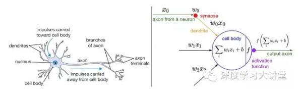
1.Sigmoid


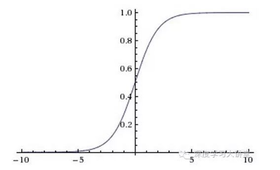
The sigmoid non-linearity has the mathematical form 


It
takes a real-valued number and “squashes” it into range between 0 and 1. In particular, large negative numbers become 0 and large positive numbers become 1. The sigmoid function has seen frequent use historically since it has a nice interpretation as the firing
rate of a neuron: from not firing at all (0) to fully-saturated firing at an assumed maximum frequency (1).
In practice, the sigmoid non-linearity has recently fallen out of favor and it is rarely ever used. It has two major drawbacks:
1. Sigmoids saturate and kill gradients. A very undesirable property of the sigmoid neuron is that when the neuron's activation saturates at either tail of 0 or 1, the gradient at these regions is almost zero.
Recall that during back-propagation, this (local) gradient will be multiplied to the gradient of this gate's output for the whole objective. Therefore, if the local gradient is very small, it will effectively “kill” the gradient and almost no signal will flow
through the neuron to its weights and recursively to its data. Additionally, one must pay extra caution when initializing the weights of sigmoid neurons to prevent saturation. For example, if the initial weights are too large then most neurons would become
saturated and the network will barely learn. 2. Sigmoid outputs are not zero-centered. This is undesirable since neurons in later layers of processing in a Neural Network (more on this soon) would be receiving data that is not zero-centered. This has implications
on the dynamics during gradient descent, because if the data coming into a neuron is always positive (e.g., x>0 element wise in

),
then the gradient on the weights w will during back-propagation become either all be positive, or all negative (depending on the gradient of the whole expression f). This could introduce undesirable zig-zagging dynamics in the gradient updates for the weights.
However, notice that once these gradients are added up across a batch of data the final update for the weights can have variable signs, somewhat mitigating this issue. Therefore, this is an inconvenience but it has less severe consequences compared to the
saturated activation problem above.

2.tanh(x)

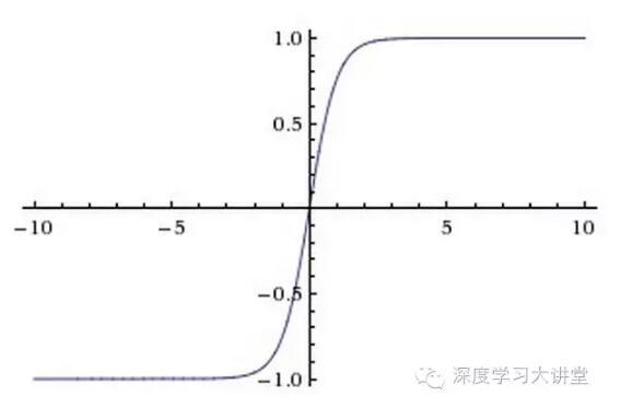
The
tanh non-linearity squashes a real-valued number to the range [-1, 1]. Like the sigmoid neuron, its activations saturate, but unlike the sigmoid neuron its output is zero-centered. Therefore, in practice the tanh non-linearity is always preferred to the sigmoid
nonlinearity.

3.Rectified Linear Unit

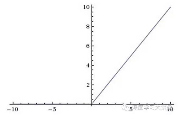
The
Rectified Linear Unit (ReLU) has become very popular in the last few years. It computes the function

,
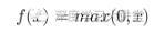
which is simply thresholded at zero.
There are several pros and cons to using the ReLUs:
1. (Pros) Compared to sigmoid/tanh neurons that involve expensive operations (exponentials, etc.), the ReLU can be implemented by simply thresholding a matrix of activations at zero. Meanwhile, ReLUs does not
suffer from saturating.
2. (Pros) It was found to greatly accelerate (e.g., a factor of 6 in [1]) the convergence of stochastic gradient descent compared to the sigmoid/tanh functions. It is argued that this is due to its linear, non-saturating
form.
3. (Cons) Unfortunately, ReLU units can be fragile during training and can “die”. For example, a large gradient flowing through a ReLU neuron could cause the weights to update in such a way that the neuron will
never activate on any datapoint again. If this happens, then the gradient flowing through the unit will forever be zero from that point on. That is, the ReLU units can irreversibly die during training since they can get knocked off the data manifold. For example,
you may find that as much as 40% of your network can be “dead” (i.e., neurons that never activate across the entire training dataset) if the learning rate is set too high. With a proper setting of the learning rate this is less frequently an issue.
4.Leaky ReLU


Leaky ReLUs are one attempt to fix the “dying ReLU”
problem. Instead of the function being zero when


, a leaky ReLU will instead have a small negative slope (of 0.01, or so).
That is, the function computes

if

and

if

,
where a is a small constant. Some people report success with this form of activation function, but the results are not always consistent.

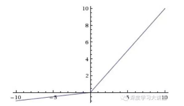
5.Parametric ReLU
Nowadays, a broader class of activation functions, namely the rectified unit family, were proposed.
In the following, we will talk about the variants of ReLU.

ReLU,
Leaky ReLU, PReLU and RReLU. In these figures, for PReLU, ai is learned and for Leaky ReLU ai is fixed. For RReLU, aji is a random variable keeps sampling in a given range, and remains fixed in testing.
The first variant is called parametric rectified linear unit (PReLU) [4]. In PReLU, the slopes of negative part are learned from data rather than pre-defined. He et al. [4] claimed that PReLU is the key factor
of surpassing human-level performance on ImageNet(http://www.image-net.org/)
classification task. The back-propagation and updating process of PReLU is very straightforward and similar to traditional ReLU, which is shown in Page. 43 of the slides.、

6.Randomized ReLU
The second variant is called randomized rectified linear unit (RReLU). In RReLU, the slopes of negative parts are randomized in a given range in the training, and then fixed in the testing. As mentioned in [5],
in a recent Kaggle National Data Science Bowl (NDSB) competition(https://www.kaggle.com/c/datasciencebowl),
it is reported that RReLU could reduce overfitting due to its randomized nature. Moreover, suggested by the NDSB competition winner, the random ai in training is sampled from

and
in test time it is fixed as its expectation, i.e.,

In
[5], the authors evaluated classification performance of two state-of-the-art CNN architectures with different activation functions on theCIFAR-10, CIFAR-100 and NDSB data sets, which are shown in the following tables. Please note that, for these two networks,
activation function is followed by each convolutional layer. And the 1/a in these tables actually indicates , where a is the aforementioned slopes.

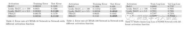
From
these tables, we can find the performance of ReLU is not the best for all the three data sets. For Leaky ReLU, a larger slope will achieve better accuracy rates. PReLU is easy to overfit on small data sets (its training error is the smallest, while testing
error is not satisfactory), but still outperforms ReLU. In addition, RReLU is significantly better than other activation functions on NDSB, which shows RReLU can overcome overfitting, because this data set has less training data than that of CIFAR-10/CIFAR-100.
In conclusion, three types of ReLU variants all consistently outperform the original ReLU in these three data sets. And PReLU and RReLU seem better choices. Moreover, He et al. also reported similar conclusions in [4].
Sec. 6: Regularizations
There are several ways of controlling the capacity of Neural Networks to prevent overfitting:
L2 regularization is perhaps the most common form of regularization. It can be implemented by penalizing the squared magnitude of all parameters directly
in the objective. That is, for every weight w in the network, we add the term

to
the objective, where

is
the regularization strength. It is common to see the factor of 1/2 in front because then the gradient of this term with respect to the parameter w is simply

instead
of

.
The L2 regularization has the intuitive interpretation of heavily penalizing peaky weight vectors and preferring diffuse weight vectors.
L1 regularization is another relatively common form of regularization, where for each weight w we add the term

to
the objective. It is possible to combine the L1 regularization with the L2 regularization:

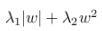
(this
is called Elastic net regularization). The L1 regularization has the intriguing property that it leads the weight vectors to become sparse during optimization (i.e. very close to exactly zero). In other words, neurons with L1 regularization end up using only
a sparse subset of their most important inputs and become nearly invariant to the “noisy” inputs. In comparison, final weight vectors from L2 regularization are usually diffuse, small numbers. In practice, if you are not concerned with explicit feature selection,
L2 regularization can be expected to give superior performance over L1.
Max norm constraints. Another form of regularization is to enforce an absolute upper bound on the magnitude of the weight vectorfor every neuron and use
projected gradient descent to enforce the constraint. In practice, this corresponds to performing the parameter update as normal, and then enforcing the constraint by clamping the weight vector

of
every neuron to satisfy

.
Typical values of c are on orders of 3 or 4. Some people report improvements when using this form of regularization. One of its appealing properties is that network cannot “explode” even when the learning rates are set too high because the updates are always
bounded.
Dropout is an extremely effective, simple and recently introduced regularization technique by Srivastava et al. in [6] that complements the other methods
(L1, L2, maxnorm). During training, dropout can be interpreted as sampling a Neural Network within the full Neural Network, and only updating the parameters of the sampled network based on the input data. (However, the exponential number of possible sampled
networks are not independent because they share the parameters.) During testing there is no dropout applied, with the interpretation of evaluating an averaged prediction across the exponentially-sized ensemble of all sub-networks (more about ensembles in the
next section). In practice, the value of dropout ratio

is
a reasonable default, but this can be tuned on validation data.

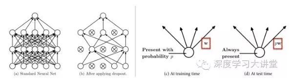
The
most popular used regularization techniquedropout [6]. While training, dropout is implemented by only keeping a neuron active with some probability p (a hyper-parameter), or setting it to zero otherwise. In addition, Google applied for a US patent(https://www.google.com/patents/WO2014105866A1)
for dropout in 2014.
Sec. 7: Insights from Figures

Finally, from the tips above, you can get the satisfactory settings (e.g., data processing, architectures choices and details, etc.) for your own deep networks. During training time, you can draw some figures
to indicate your networks’ training effectiveness.
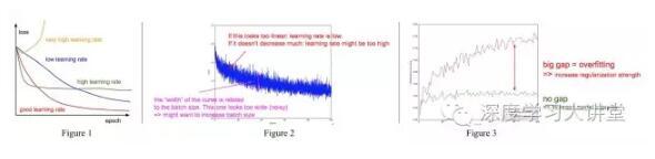
1. As we have known, the learning rate is very sensitive. From Fig. 1 in the following, a very high learning rate will cause a quite strange loss curve. A low learning rate will make your training loss decrease
very slowly even after a large number of epochs. In contrast, a high learning rate will make training loss decrease fast at the beginning, but it will also drop into a local minimum. Thus, your networks might not achieve a satisfactory results in that case.
For a good learning rate, as the red line shown in Fig. 1, its loss curve performs smoothly and finally it achieves the best performance.

2. Now let’s zoom in the loss curve. The epochs present the number of times for training once on the training data, so there are multiple mini batches in each epoch. If we draw the classification loss every
training batch, the curve performs like Fig. 2. Similar to Fig. 1, if the trend of the loss curve looks too linear, that indicates your learning rate is low; if it does not decrease much, it tells you that the learning rate might be too high. Moreover, the
“width” of the curve is related to the batch size. If the “width” looks too wide, that is to say the variance between every batch is too large, which points out you should increase the batch size.
3. Another tip comes from the accuracy curve. As shown in Fig. 3, the red line is the training accuracy, and the green line is the validation one. When the validation accuracy converges, the gap between the
red line and the green one will show the effectiveness of your deep networks. If the gap is big, it indicates your network could get good accuracy on the training data, while it only achieve a low accuracy on the validation set. It is obvious that your deep
model overfits on the training set. Thus, you should increase the regularization strength of deep networks. However, no gap meanwhile at a low accuracy level is not a good thing, which shows your deep model has low learnability. In that case, it is better
to increase the model capacity for better results.


Sec. 8: Ensemble
In machine learning, ensemble methods [8] that train multiple learners and then combine them for use are a kind of state-of-the-art learning approach. It is well known that an ensemble is usually significantly
more accurate than a single learner, and ensemble methods have already achieved great success in many real-world tasks. In practical applications, especially challenges or competitions, almost all the first-place and second-place winners used ensemble methods.Here
we introduce several skills for ensemble in the deep learning scenario.
Same model, different initialization. Use cross-validation to determine the best hyperparameters, then train multiple models with the best set of hyperparameters
but with different random initialization. The danger with this approach is that the variety is only due to initialization. Top models discovered during cross-validation. Use
cross-validation to determine the best hyperparameters, then pick the top few (e.g., 10) models to form the ensemble. This improves the variety of the ensemble but has the danger of including suboptimal models. In practice, this can be easier to perform since
it does not require additional retraining of models after cross-validation. Actually, you could directly select several state-of-the-art deep models from Caffe Model Zoo (https://github.com/BVLC/caffe/wiki/Model-Zoo)
to perform ensemble. Different checkpoints of a single model. If training is very expensive, some people have had limited success in taking different
checkpoints of a single network over time (for example after every epoch) and using those to form an ensemble. Clearly, this suffers from some lack of variety, but can still work reasonably well in practice. The advantage of this approach is that is very cheap. Some
practical examples. If your vision tasks are related to high-level image semantic, e.g., event recognition from still images, a better ensemble method is to employ multiple deep models trained on different
data sources to extract different and complementary deep representations. For example in the Cultural Event Recognition (https://www.codalab.org/competitions/4081#learn_the_details)
challenge in associated with ICCV’15 (http://pamitc.org/iccv15/)
, we utilized five different deep models trained on images of ImageNet (http://www.image-net.org/),
Place Database (http://places.csail.mit.edu/)
and the cultural images supplied by the competition organizers (http://gesture.chalearn.org/).
After that, we extracted five complementary deep features and treat them as multi-view data. Combining “early fusion” and “late fusion” strategies described in [7], we achieved one of the best performance and ranked the 2nd place in that challenge. Similar
to our work, [9] presented the Stacked NN framework to fuse more deep networks at the same time.
References & Source Links
[1] A. Krizhevsky, I. Sutskever, and G. E. Hinton. ImageNet Classification with Deep Convolutional Neural Networks.(http://papers.nips.cc/paper/4824-imagenet-classification-with-deep-convolutional-neural-networks.pdf)
In NIPS, 2012
[2] A Brief Overview of Deep Learning (http://yyue.blogspot.com/2015/01/a-brief-overview-of-deep-learning.html/)
, which is a guest post by Ilya Sutskever.
[3] CS231n: Convolutional Neural Networks for Visual Recognition of Stanford University, held by Prof. Fei-Fei Li and Andrej Karpathy.
[4] K. He, X. Zhang, S. Ren, and J. Sun. Delving Deep into Rectifiers: Surpassing Human-Level Performance on ImageNet Classification.（http://arxiv.org/abs/1502.01852）InICCV,
2015.
[5] B. Xu, N. Wang, T. Chen, and M. Li. Empirical Evaluation of Rectified Activations in Convolution Network（http://arxiv.org/abs/1505.00853）.
In ICML Deep Learning Workshop, 2015.
[6] N. Srivastava, G. E. Hinton, A. Krizhevsky, I. Sutskever, and R. Salakhutdinov. Dropout: A Simple Way to Prevent Neural Networks from Overfitting. （http://jmlr.org/papers/v15/srivastava14a.html）JMLR,
15(Jun):1929−1958, 2014.
[7] X.-S. Wei, B.-B. Gao, and J. Wu. Deep Spatial Pyramid Ensemble for Cultural Event Recognition. （http://lamda.nju.edu.cn/weixs/publication/iccvw15_CER.pdf）In
ICCV ChaLearn Looking at People Workshop, 2015.
[8] Z.-H. Zhou. Ensemble Methods: Foundations and Algorithms（https://www.crcpress.com/Ensemble-Methods-Foundations-and-Algorithms/Zhou/9781439830031）.
Boca Raton, FL: Chapman & HallCRC/, 2012. (ISBN 978-1-439-830031)
[9] M. Mohammadi, and S. Das. S-NN: Stacked Neural Networks. Project in Stanford CS231n Winter Quarter, 2015.（http://cs231n.stanford.edu/reports/milad_final_report.pdf）
[10] P. Hensman, and D. Masko. The Impact of Imbalanced Training Data for Convolutional Neural Networks.（http://www.diva-portal.org/smash/get/diva2:811111/FULLTEXT01.pdf）
Degree Project in Computer Science, DD143X, 2015.