Neural Networks and Deep Learning CH2
2016-10-14 11:23
543 查看
Warm up a fast matrix-based approach to computing the output from a neural network
The two assumptions we need about the cost function
The Hadamard product
Backpropagation
The four fundamental equations behind backpropagation
Proof of the four fundamental equations
My summary
The backpropagation algorithm
In what sense is backpropagation a fast algorithm
Backpropagation the big picture
这一章主要介绍了backpropagation算法的原理。
backpropagation的核心是一个计算∂C∂w的表达式。其中C为cost function,参数是weight w,bias b。这个表达式告诉我们当我们改变weight和bias的时候,cost function的改变有多快。
这些定义和之前学的没什么不同。
如下图:
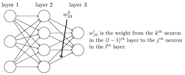
然后解释了为什么定义wljk是第l层第j个神经元和第l−1层第k个神经元的weight:
这样定义可以在向量化的时候去掉一个转置符号,公式漂亮且加快了运算速度。
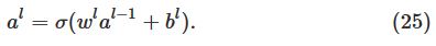
其中cost function C为:
L表示神经网络的层数。aL即输出层。
为了backpropagation能工作,我们需要做出以下两个主要的假设:
第一,cost function对于每一个训练样例x的Cx,能够写成均值形式C=1n∑xCx。需要这个假设的原因是backpropagation实际上是先对单独的训练样例x计算∂Cx∂w和∂Cx∂w,之后再用均值来算总的。
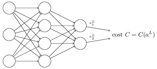
第二,cost function能够被写成神经网络输出的函数,如下图:
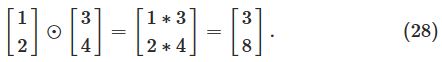
含义是elementwise的乘法运算,如下图例子:
首当其冲要明白,算法的目的是计算∂C∂w和∂C∂b。
而∂C∂b的计算方法可以由∂C∂w的证明中得出来,因此先写出∂C∂w,就可以轻易写出∂C∂b。
以下是关于∂C∂w的计算过程和证明过程:
首先,由于:
根据chain rule,可以写出:
∂C∂wlij=∂zli∂wlij∂C∂zli。
对于等式右边第一项∂zli∂wlij:
由于zli=∑jwlijal−1j,因此∂zli∂wlij=al−1j(输入定义为a0)。
对于等式右边第二项∂C∂zli:
定义δli=∂C∂zli。
对于输出层:
根据chain rule,可以写出:
δLj=∂aLj∂zLj∂C∂aLj=∂C∂aLjσ′(zLj)(输出定义为aL)。
又由于:
根据chain rule,可以写出:
δli=∂C∂zli=∂ali∂zli∑k∂zl+1k∂ali∂C∂zl+1k
上式右边第一项:∂ali∂zli=σ′(zlj)。
上式右边第二项:zl+1k=∑iwl+1kiali+bl+1k。
所以,∂zl+1k∂ali=wl+1ki。
上式右边第三项:∂C∂zl+1k=δl+1k。
综上,得到第l+1层到第l层的δ递推式,原来求的初始条件L也有了意义。
其递推式为:δli=σ′(zli)∑kwl+1kiδl+1k,将其矩阵化,可以得到:δl=((wl+1)Tδl+1)⊙σ′(zl)。
至此,所有关于∂C∂w的计算过程和证明过程结束。可以得到以下三个重要公式:
δLj=∂C∂aLjσ′(zLj)
δl=((wl+1)Tδl+1)⊙σ′(zl)
∂C∂wlij=al−1jδli
同理,用链式法则可以得到最后一个重要公式:
∂C∂blj=δlj
至此,整个backpropagation简单版的推导与公式计算就此结束。
具体实现,上一章有完整代码:
朴素的算法是对于每一个weight,计算一次偏导,那么当整个神经网络的神经元个数非常多的时候,这个计算量就非常大了。而backpropagation快就在于它能够一次前向传播,一次后向传播计算出所有的偏导。
其一,这个算法在我们做这些矩阵与向量乘法的时候,究竟做了什么。
其二,第一个发现这个算法的人是如何发现它的。
对于第一个问题:
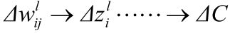
首先假设我们对weight wljk做了一个小改变:
这个改变将会导致接下来一个神经元的输入的改变:
然后继续依此影响接下来的每一层:
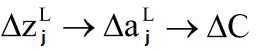
直到影响到输出,以及cost function:
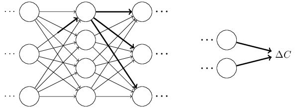
cost function的改变可以由一下式子给出:
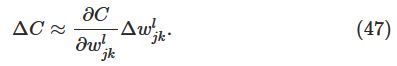
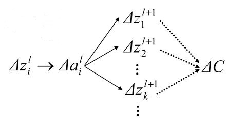
这个式子说明计算出∂C∂wljk,就可以计算出改变weight对cost function的影响。由类似chain rule的一系列运算,可以得到:
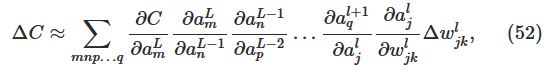
因此:

其实意义就是,backpropagation提供了一种计算以上所有影响了cost function路径的和。记录了这些路径的改变是如何影响到输出层和cost function的。
事实上,第二个问题也是由上述过程发现的,也就是说,第一个发现backpropagation的人也是按照以上流程发现了这种算法,而其原来的证明非常复杂,以上的证明只是简单版本的。
The two assumptions we need about the cost function
The Hadamard product
Backpropagation
The four fundamental equations behind backpropagation
Proof of the four fundamental equations
My summary
The backpropagation algorithm
In what sense is backpropagation a fast algorithm
Backpropagation the big picture
这一章主要介绍了backpropagation算法的原理。
backpropagation的核心是一个计算∂C∂w的表达式。其中C为cost function,参数是weight w,bias b。这个表达式告诉我们当我们改变weight和bias的时候,cost function的改变有多快。
Warm up: a fast matrix-based approach to computing the output from a neural network
这一节回顾了一个基于矩阵的计算神经网络输出的算法。并对一些backpropagation用到的符号进行了定义。这些定义和之前学的没什么不同。
如下图:
然后解释了为什么定义wljk是第l层第j个神经元和第l−1层第k个神经元的weight:
这样定义可以在向量化的时候去掉一个转置符号,公式漂亮且加快了运算速度。
The two assumptions we need about the cost function
Backpropagation的目标是计算在网络中的任意∂C∂w和∂C∂b。其中cost function C为:
L表示神经网络的层数。aL即输出层。
为了backpropagation能工作,我们需要做出以下两个主要的假设:
第一,cost function对于每一个训练样例x的Cx,能够写成均值形式C=1n∑xCx。需要这个假设的原因是backpropagation实际上是先对单独的训练样例x计算∂Cx∂w和∂Cx∂w,之后再用均值来算总的。
第二,cost function能够被写成神经网络输出的函数,如下图:
The Hadamard product
这一节介绍了一个运算符号s⊙t。含义是elementwise的乘法运算,如下图例子:
Backpropagation
The four fundamental equations behind backpropagation
这一节是关于backpropagation的重要的四个公式,是这一章的核心。Proof of the four fundamental equations
这一节简单介绍了公式的推导。My summary
感觉这两节的写法以及证明方法没有NTU课堂上的逻辑清晰,结合二者,我自己总结了一下。证明全是基于chain rule。首当其冲要明白,算法的目的是计算∂C∂w和∂C∂b。
而∂C∂b的计算方法可以由∂C∂w的证明中得出来,因此先写出∂C∂w,就可以轻易写出∂C∂b。
以下是关于∂C∂w的计算过程和证明过程:
首先,由于:
根据chain rule,可以写出:
∂C∂wlij=∂zli∂wlij∂C∂zli。
对于等式右边第一项∂zli∂wlij:
由于zli=∑jwlijal−1j,因此∂zli∂wlij=al−1j(输入定义为a0)。
对于等式右边第二项∂C∂zli:
定义δli=∂C∂zli。
对于输出层:
根据chain rule,可以写出:
δLj=∂aLj∂zLj∂C∂aLj=∂C∂aLjσ′(zLj)(输出定义为aL)。
又由于:
根据chain rule,可以写出:
δli=∂C∂zli=∂ali∂zli∑k∂zl+1k∂ali∂C∂zl+1k
上式右边第一项:∂ali∂zli=σ′(zlj)。
上式右边第二项:zl+1k=∑iwl+1kiali+bl+1k。
所以,∂zl+1k∂ali=wl+1ki。
上式右边第三项:∂C∂zl+1k=δl+1k。
综上,得到第l+1层到第l层的δ递推式,原来求的初始条件L也有了意义。
其递推式为:δli=σ′(zli)∑kwl+1kiδl+1k,将其矩阵化,可以得到:δl=((wl+1)Tδl+1)⊙σ′(zl)。
至此,所有关于∂C∂w的计算过程和证明过程结束。可以得到以下三个重要公式:
δLj=∂C∂aLjσ′(zLj)
δl=((wl+1)Tδl+1)⊙σ′(zl)
∂C∂wlij=al−1jδli
同理,用链式法则可以得到最后一个重要公式:
∂C∂blj=δlj
至此,整个backpropagation简单版的推导与公式计算就此结束。
The backpropagation algorithm
mini-batch的伪代码:具体实现,上一章有完整代码:
def backprop(self, x, y):
"""Return a tuple "(nabla_b, nabla_w)" representing the
gradient for the cost function C_x.  "nabla_b" and
"nabla_w" are layer-by-layer lists of numpy arrays, similar
to "self.biases" and "self.weights"."""
nabla_b = [np.zeros(b.shape) for b in self.biases]
nabla_w = [np.zeros(w.shape) for w in self.weights]
# feedforward
activation = x
activations = [x] # list to store all the activations, layer by layer
zs = [] # list to store all the z vectors, layer by layer
for b, w in zip(self.biases, self.weights):
z = np.dot(w, activation)+b
zs.append(z)
activation = sigmoid(z)
activations.append(activation)
# backward pass
delta = self.cost_derivative(activations[-1], y) * \
sigmoid_prime(zs[-1])
nabla_b[-1] = delta
nabla_w[-1] = np.dot(delta, activations[-2].transpose())
# Note that the variable l in the loop below is used a little
# differently to the notation in Chapter 2 of the book.  Here,
# l = 1 means the last layer of neurons, l = 2 is the
# second-last layer, and so on.  It's a renumbering of the
# scheme in the book, used here to take advantage of the fact
# that Python can use negative indices in lists.
for l in xrange(2, self.num_layers):
z = zs[-l]
sp = sigmoid_prime(z)
delta = np.dot(self.weights[-l+1].transpose(), delta) * sp
nabla_b[-l] = delta
nabla_w[-l] = np.dot(delta, activations[-l-1].transpose())
return (nabla_b, nabla_w)
In what sense is backpropagation a fast algorithm?
这一节解释了为什么backpropagation计算∂C∂wj的速度比较快。朴素的算法是对于每一个weight,计算一次偏导,那么当整个神经网络的神经元个数非常多的时候,这个计算量就非常大了。而backpropagation快就在于它能够一次前向传播,一次后向传播计算出所有的偏导。
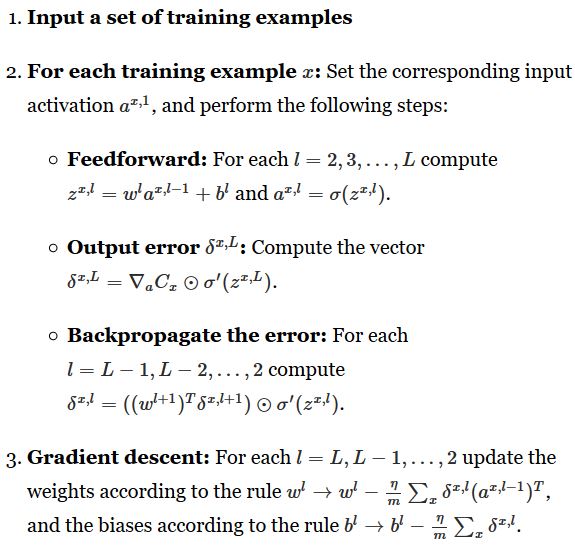
Backpropagation: the big picture
这一节解释了两个问题:其一,这个算法在我们做这些矩阵与向量乘法的时候,究竟做了什么。
其二,第一个发现这个算法的人是如何发现它的。
对于第一个问题:
首先假设我们对weight wljk做了一个小改变:
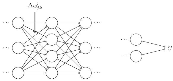
这个改变将会导致接下来一个神经元的输入的改变:
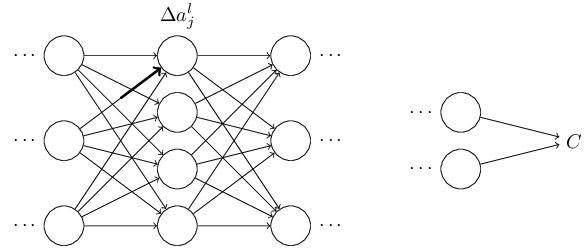
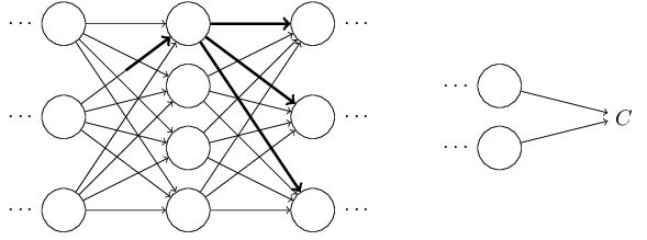
然后继续依此影响接下来的每一层:
直到影响到输出,以及cost function:
cost function的改变可以由一下式子给出:
这个式子说明计算出∂C∂wljk,就可以计算出改变weight对cost function的影响。由类似chain rule的一系列运算,可以得到:
因此:
其实意义就是,backpropagation提供了一种计算以上所有影响了cost function路径的和。记录了这些路径的改变是如何影响到输出层和cost function的。
事实上,第二个问题也是由上述过程发现的,也就是说,第一个发现backpropagation的人也是按照以上流程发现了这种算法,而其原来的证明非常复杂,以上的证明只是简单版本的。

相关文章推荐
- Neural Networks and Deep Learning(一)
- Neural Networks and Deep Learning 学习笔记(一)
- Neural Networks and Deep Learning之中文翻译-关于练习与问题
- Neural Networks and Deep Learning 学习笔记
- Neural Networks and Deep Learning之中文翻译-第一章 用神经网络识别手写数字
- Coursera-Deep Learning Specialization 课程之(一):Neural Networks and Deep Learning-weak1
- Andrew Ng-Neural Networks and Deep Learning 第二周作业
- neural networks and deep learning(Michael Nielsen)笔记(1)
- Neural Networks and Deep Learning系列(一)概述
- 神经网络与深度学习( Neural Networks and Deep Learning)
- Andrew Ng-Neural Networks and Deep Learning 第四周作业【2】
- 【deeplearning.ai】Neural Networks and Deep Learning——深层神经网络
- 【吴恩达 Coursera深度学习课程】 Neural Networks and Deep Learning 第一周课后习题
- 神经⽹络与深度学习 Neural Networks and Deep Learning
- Neural Networks and Deep Learning-读书笔记
- Neural Networks and Deep Learning之中文翻译-随记
- Neural Networks and Deep Learning 学习笔记(七)
- 读书笔记--Neural Networks and Deep Learning(CH1)
- neural networks and deep learning 吴恩达coursera公开课
- Neural Networks and Deep Learning之中文版翻译-前言