Machine Learning Basics（要点）

目录：

Machine Learning Basics
Learning Algorithms
The Task T

The Performance Measure P

The Experience E

Example Linear Regression

Generalization Capacity Overfitting and Underfitting
The No Free Lunch Theorem

Regularization

Hyperparameters and Validation Sets
Cross-Validation

Estimators Bias and Variance
Point Estimation
Function Estimation

Bias
Example Bernoulli Distribution

Example Gaussian Distribution Estimator of the Mean

Example Gaussian Distribution Estimators of the Variance

Variance
Example Bernoulli Distribution

Example Gaussian Distribution Estimators of the Variance

Trading off Bias and Variance and the Mean Squared Error
Example Gaussian Distribution Estimators of the Variance

Consistency

Maximum Likelihood Estimation
Conditional Log-Likelihood and Mean Squared Error

Properties of Maximum Likelihood

Bayesian Statistics

Maximum A Posteriori MAP Estimation

Supervised Learning Algorithms
Probabilistic Supervised Learning

Support Vector Machines

Other Simple Supervised Learning Algorithms

Unsupervised Learning Algorithms
Principal Components Analysis

Weakly Supervised Learning

Building a Machine Learning Algorithm

Machine Learning Basics

原文

@unpublished{
Bengio-et-al-2015-Book,
title={
Deep Learning
},
author={
Yoshua Bengio and Ian J. Goodfellow and Aaron Courville
},
note={
Book in preparation for MIT Press
},
url={ http://www.iro.umontreal.ca/~bengioy/dlbook },
year={
2015
}
}

Learning Algorithms

“A computer program is said to learn from experience E with respect to some class of tasks T and performance measure P , if its performance at tasks in T , as measured by P , improves with experience E”

The Task, T

Classification：f:Rn→{1,...,k}；to specify which of k categories some input belongs to.

Classification：where f outputs a probability distribution over classes.

Classification with missing inputs：…

Regression：f:Rn→R；An example of a regression task is the prediction of the expected claim amount that an insured person will make (used to set insurance premia), or the prediction of future prices of securities.

Transcription：…

Translation：…

Structured output ：…

Anomaly detection：sifts througha set of events or objects, and flags some of them as being unusual or atypical.

Synthesis and sampling：generate new examples that are similar to those in the training data.

Imputation of missing values：…

Denoising：…

Density or probability function estimation：learn a function pmodel:Rn→R.

The Performance Measure, P

For tasks such as classification, classification with missing inputs, and tran-scription, we often measure the accuracy of the model.

We often refer tothe error rate as the expected 0-1 loss. The 0-1 loss on a particular example is 0if it is correctly classified and 1 if it is not.

For tasks such as density estimation,we can measure the probability the model assigns to some examples.

The Experience, E

Machine learning algorithms can be broadly categorized as unsupervised or supervised.

Unsupervised learning algorithms experience a dataset containing many features, then learn useful properties of the structure of this dataset, to learn the probability distribution p(x).

In the contextof deep learning, we usually want to learn the entire probability distribution that generated a dataset.

Supervised learning involves observing several examples of a random vector x and an associated value or vector y, and learning to predict y from x, e.g. estimating p(y∣x).

The joint distribution can be decomposed as p(x)=Πni=1p(xi∣x1,...,xi−1). This decomposition means that we can solve the ostensibly unsupervised problem of modeling p(x) by splitting it into n supervised learning problems.

One common way of describing a dataset is with a design matrix. A design matrix is a matrix containing a different example in each row. Each column of the matrix corresponds to a different feature.

Example: Linear Regression

Take a vector x∈Rn as input and predict the value of a scalar y∈R as its output.

y^=wTx+b, where w∈Rn is a vector of parameters, b is an intercept term.

Task T : to predict y from x by outputting y^=wTx+b.

One way of measuring the performance of the model is to compute the mean squared error of the model on the test set.

the mean squared error on the test set is given by MSEtest=1m∑i(y^(test)−y(test))2i.

We can also see that, MSEtest=1m∣∣y^(test)−y(test)∣∣22.

To minimize MSEtrain, we can simply solve for where its gradient is 0: ∇wMSEtrain=0.

⇒w=(X(train)TX(train))−1X(train)Ty(train), known as the normal equations.

Generalization, Capacity, Overfitting and Underfitting

the train error: 1m(train)∣∣X(train)w−y(train)∣∣22

the test error: 1m(test)∣∣X(test)w−y(test)∣∣22

If the training and the test set are collected arbitrarily, there is indeed little we can do. If we are allowed to make some assumptions about how the training and testset are collected, then we can make some progress.

the examples in each dataset are independent from each other, and that the train set and test set are identically distributed, drawn from the same probability distribution as each other.

The factors determining how well a machine learning algorithm will perform are its ability to:

Make the training error small.

Make the gap between training and test error small.

Underfitting occurs when the model is not able to obtain a sufficiently low error value on the training set. Overfitting occurs when the gap between the training error and test error is too large.

We can control whether a model is more likely to overfit or underfit by altering its capacity.

One way to control the capacity of a learning algorithm is by choosing its hypothesis space.

Occam′srazor:

among competing hypotheses that explain known observations equally well, one should choose the “simplest” one.

the discrepancy between training error and generalization error is bounded by a quantity that grows with the ratio of capacity to number of training examples.

To reach the most extreme case of arbitrarily high capacity, we introduce the concept of non-parametric models.

One example of such an algorithm is nearest neighbor regression => y^=yi where i=argmin||Xi,:−x||22.

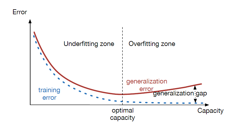
Figure 5.3: Typical relationship between capacity (horizontal axis) and both training(bottom curve, dotted) and generalization (or test) error (top curve, bold):



We can also create a non-parametric learning algorithm by wrapping a parametric learning algorithm inside another algorithm that increases the number of parameters as needed. For example, we could imagine an outer loop of learning that changes the degree of the polynomial learned by linear regression on top of a polynomial expansion of the input.

The error incurred by an oracle making predictions from the true distribution p(x, y) is called the Bayes error.

The model specifies which family of functions the learning algorithm can choose from when varying the parameters in order to reduce a training objective.This is called the representational capacity of the model.

In practice, the learning algorithm does not actually find the best function, just one that significantly reduces the training error. => effective capacity.

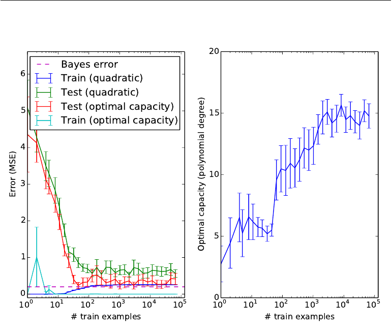
Figure 5.4: The effect of the training dataset size on the train and test error of the model,as well as on the optimal model capacity:

The No Free Lunch Theorem

Machine learning avoids this problem by offering only probabilistic rules, rather than the entirely certain rules used in purely logical reasoning. Machine learning promises to find rules that are probably correct about most members of the set they concern.

The goal of machine learning research is not to seek a universal learning algorithm or the absolute best learning algorithm. Instead, the goal is to understand what kinds of distributions are relevant to the “real world” that an AI agent experiences, and what kinds of machine learning algorithms perform well on data drawn from the kinds of data generating distributions that are care about.

Regularization

Modify the training criterion for linear regression to include weight decay.

J(w)=MSEtrain+λwTw

Minimizing J(w) results in a choice of weights that make a trade off between fitting the training data and being small.

Regularization is any modification we make to a learning algorithm that is intended to reduce its generalization error but not its training error.

Hyperparameters and Validation Sets

Most machine learning algorithms have several settings that we can use to control the behavior of the learning algorithm. These settings are called hyperparameters.

We do not learn the hyper-parameter because it is not appropriate to learn that hyper-parameter on the training set. This applies to all hyper-parameters that control model capacity.

To solve this problem, we need a validation set of examples that the training algorithm does not observe.

We always construct the validation set from the training data. Specifically, we split the training data into two disjoint subsets. One of these subsets is used to learn the parameters. The other subset is our validation set,used to estimate the generalization error during or after training, allowing for the hyper-parameters to be updated accordingly.

The validation set is used to “train” the hyper-parameters.

Typically, one uses about 80% of the data for training and 20% for validation.

Cross-Validation

The K-Fold Cross-Validation Procedure: A partition of the dataset is formed by splitting it in k non-overlapping subsets, then k train/test splits can be obtained by keeping each time the i-th subset as a test set and the rest as a training set. The average test error across all these k training/testing experiments can then be reported.

One problem is that there exists no unbiased estimators of the variance of such average error estimators , but approximations are typically used.

If model selection or hyper-parameter optimization is required, things get more computationally expensive: one can recurse the k-fold cross-validation idea, in-side the training set.:

we can have an outer loop that estimates test error and provides a “training set” for a hyper-parameter-free learner, calling it k times to“train”. That hyper-parameter-free learner can then split its received training set by k-fold cross-validation into internal training/validation subsets (for example,splitting into k − 1 subsets is convenient, to reuse the same test blocks as the outer loop), call a hyper-parameter-specific learner for each choice of hyper-parameter value on each of the training partition of this inner loop, and compute the validation error by averaging across the k −1 validation sets the errors made by the k −1 hyper-parameter-specific learners trained on each of the internal training subsets.

Estimators, Bias and Variance

Point Estimation

Let {x(1),...,x(m)} be a set of m independent and identically distributed(i.i.d.) data points. A point estimator is any function of the data: θ^m=g(x(1),...,x(m)). In other words, any statistic is a point estimate.

For now, we take the frequentist perspective on statistics. That is, we assume that the true parameter value θ is fixed but unknown, while the point estimate θ^ is a function of the data. Since the data is drawn from a random process, any function of the data is random. Therefore θ^ is a random variable.

Function Estimation

To predict a variable (or vector) y given an input vector x (also called the covariates), considering that there is a function f(x) that describes the relationship between yand x.

The function estimator f^ is simply a point estimator in function space.

When we discuss properties of the estimator, we are really describing properties of the sampling distribution.

Bias

The bias of an estimator is defined as: bias(θ^m)=E(θ^m)−θ

An estimator θ^ is said to be unbiased if bias(θ^m)=0, i.e., if E(θ^m)=θ. An estimator θ^ is said to be asymptotically unbiased if limm→∞bias(θ^m)=0,i.e., if limm→∞E(θ^m)=θ.

Example: Bernoulli Distribution

Consider a set of samples {x(1),...,x(m)} that are independently and identically distributed according to a Bernoulli distribution, x(i)∈0,1, where i∈[1,m]. The Bernoulli p.m.f. (probability massfunction, or probability function) is given by P(x(i);θ)=θx(i)(1−θ)(1−x(i)) .

The estimator θ^m=1m∑mi=1x(i) .

Bias(θ^)=0, we say that our estimator θ^ is unbiased.

Example: Gaussian Distribution Estimator of the Mean

Consider a set of samples {x(1),...,x(m)} that are independently and identically distributed according to a Gaussian (Normal) distribution (x(i)∼Gaussian(μ,σ2), where i∈[1,m]). The Gaussian p.d.f. (probability density function) is given by p(x(i);μ,σ2)=12πσ2√exp(−12(x(i)−μ)2σ2).

The sample mean: μ^m=1m∑mi=1x(i) is an unbiased estimator of Gaussian mean parameter.

Example: Gaussian Distribution Estimators of the Variance

The sample variance: σ^2m=1m∑mi=1(x(i)−μ^m)2

The bias of σ^2m is −σ2/m. Therefore, the sample variance is a biased estimator.

The unbiased sample variance: σ~2m=1m−1∑mi=1(x(i)−μ^m)2

While unbiased estimators are clearly desirable, they are not always the “best” estimators. As we will see we often use biased estimators that possess other important properties.

Variance

Variance: Var(θ^)=E[θ^2]−E[θ^]2.

Standard error (se) of the estimator: se(θ^)=Var[θ^]−−−−−√.

Example: Bernoulli Distribution

The variance of the estimator θ^m=1m∑mi=1x(i): Var(θ^)=1mθ(1−θ)

The variance of the estimator decreases as a function of m, the number of examples in the dataset.

Example: Gaussian Distribution Estimators of the Variance

Relationship between the sample variance and the Chi Squared distribution, specifically, that m−1σ2σ^2 happens to be χ2 distributed.

The variance of a χ2 random variable with m−1 degrees of freedom is 2(m−1).

The sample variance: Var(σ^2)=2(m−1)σ4m2.

The unbiased sample variance: Var(σ~2)=2σ4(m−1)

So while the bias of σ~2 is smaller than the bias of σ^2, the variance of σ~2 is greater.

Trading off Bias and Variance and the Mean Squared Error

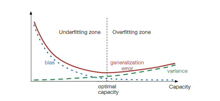
Bias and variance measure two different sources of error in an estimator. Bias measures the expected deviation from the true value of the function or parameter. Variance on the other hand, provides a measure of the deviation from the true value that any particular sampling of the data is likely to cause.

To negotiate this kind of trade-off, in general is by cross-validation, discussed in Section cross-validation.

We can also compare the mean squared error (MSE)of the estimates: MSE=E[(θ^n−θ)2]=Bias(θ^n)2+Var(θ^).

In the case where generalization error is measured by the MSE (where bias and variance are meaningful components of generalization error), increasing capacity tends to increase variance and decrease bias.

Example: Gaussian Distribution Estimators of the Variance

MSE(σ^2m)=Bias(σ^2m)2+Var(σ^2m)=(2m−1m2)σ4

MSE(σ~2m)=Bias(σ~2m)2+Var(σ~2m)=2(m−1)σ4

Comparing the two, we see that the MSE of the unbiased sample variance, σ~2m, is actually higher than the MSE of the (biased) sample variance, σ^2m. This implies that despite incurring bias in the estimator σ^2m, the resulting reduction in variance more than makes up for the difference, at least in a mean squared sense.

Consistency

We might wish that, as the number of data points in our dataset increases, our point estimates converge to the true value of the parameter. More formally, we would like that limn→∞θn^−→pθ.

This condition is known as consistency.

Asymptotic unbiasedness is not equivalent to consistency.

For example, consider estimating the mean parameter μ of a normal distribution N(μ,σ2), with a dataset consisting of n samples: {x1,...,xn}. We could use the first sample x1 of the dataset as an unbiased estimator: θ^=x1, In that case, E(θ^n)=θ so the estimator is unbiased no matter how many data points are seen. This, of course, implies that the estimate is asymptotically unbiased. However, this is not a consistent estimator as it is not the case that θ^n→θ as n→∞.

Maximum Likelihood Estimation

We would like to have some principle from which we can derive specific functions that are good estimators for different models. The most common such principle is the maximum likelihood principle.

The maximum likelihood estimator for θ is then defined as:

θML=argmaxθpmodel(X;θ)=argmaxθ∏mi=1pmodel(x(i);θ)

Expressed as an expectation:

θML=argmaxθEx∼p^datalogpmodel(x;θ)

The KL divergence is given by

DKL(p^data||pmodel)=Ex∼p^data[logp^data(x)−logpmodel(x)]

We can thus see maximum likelihood as an attempt to make the model distribution match the empirical distribution p^data.

Conditional Log-Likelihood and Mean Squared Error

The conditional maximum likelihood estimator is：

θML=argmaxθP(Y∣X;θ).

Assumed to be i.i.d. ：

θML=argmaxθ∑mi=1logP(y(i)∣x(i);θ).

Properties of Maximum Likelihood

There is the question of how many training examples one needs to achieve a particular generalization error, or equivalently what estimation error one gets for a given number of training examples, also called efficiency.

A way to measure how close we are to the true parameter is by the expected mean squared error.

For m large, no consistent estimator has a lower mean squared error than the maximum likelihood estimator.

Bayesian Statistics

The frequentist perspective is that the true parameter value θ is fixed but unknown, while the point estimate θ^ is a random variableon account of it being a function of the data (which are seen as random).

The Bayesian uses probability to reflect degrees of certainty ofstates of knowledge. The data is directly observed and so is not random. On the other hand, the true parameter θ is unknown or uncertain and thus is represented as a random variable.

Bayesian statistics provides a natural and theoretically elegant way to consider all possible values of θ when making a prediction.

Before observing the data, we represent our knowledge of θ using the prior probability distribution, p(θ).

Unlike the maximum likelihood point estimate of θ, the Bayesian makes decision with respect to a full distribution over θ.

p(x(m+1)∣x(1),...,x(m))=∫p(x(m+1)∣θ)p(θ∣x(1),...,x(m))dθ

The Bayesian answer to the question of how to deal with the uncertainty in the estimator is to simply integrate over it, which tends to protect well against overfitting.

Combining the prior, p(θ), with the data likelihood p(x(1),...,x(m)∣θ) results in a distribution that is less entropic (more peaky)than the prior. This is just the result of a basic property of probability distributions: Entropy(product oftwo densities)≤Entropy(either density). This implies that the posterior density on θ is also less entropic than the data likelihood alone(when viewed and normalized as a density over θ).

The hypothesis space with the Bayesian approach is, to some extent, more constrained than that with an ML approach. Thus we expect a contribution of the prior to be a further reduction in overfitting as compared to ML estimation.

Maximum A Posteriori (MAP) Estimation

The MAP estimate chooses the point of maximal posterior probability (or maximal probability density in the more common case of continuous θ):

θMAP=argmaxθ p(θ∣x)=argmaxθ logp(x∣θ)+logp(θ)

Introducing the infuence of the prior on the MAP estimate helps to reduce the variance in the MAP point estimate (in comparison to the ML estimate). However, it does so at the price of increased bias.

As the variance of the prior distribution tends to infinity, the MAP estimate reduces to the ML estimate. As the variance of the prior tends to zero,the MAP estimate tends to zero (actually it tends to µ0which here is assumedto be zero).

The incurred bias is a consequence of the reduction in model capacity caused by limiting the space of hypotheses to those with significant probability density under the prior.

Many regularized estimation strategies, such as maximum likelihood learning regularized with weight decay, can be interpreted as making the MAP approximation to Bayesian inference. This view applies when the regularization consists of adding an extra term to the objective function that corresponds to logp(θ).

Supervised Learning Algorithms

Probabilistic Supervised Learning

Most supervised learning algorithms in this book are based on estimating a probability distribution p(y∣x).

Linear regression corresponds to the family p(y∣x;θ)=N(y∣θTx,I).

Logistic regression corresponds to the family p(y=1∣x;θ)=σ(θTx).

Support Vector Machines

This model is similar to logistic regression in that it is driven by a linear function wTx+b. Unlike logistic regression, the support vector machine does not provide probabilities, but only outputs a class identity.

One key innovation associated with support vector machines is the kernel trick:

k(x,x(i))=ϕ(x)Tϕ(x(i))

The linear function used by the support vector machine can be re-written as wTx+b=b+∑mi=1αixTx(i).

We can then make predictions using the function f(x)=b+∑iαik(x,x(i)). This function is linear in the space that ϕ maps to, but non-linear as a function of x.

The kernel trick is powerful for two reasons:

First, it allows us to learn models that are non-linear as a function of x using convex optimization techniques that are guaranteed to converge efficiently. This is only possible because we consider ϕ fixed and only optimize α.

Second, the kernel function k need not be implemented in terms of explicitly applying the ϕ mapping and then applying the dot product. The dot product in ϕ space might be equivalent to a non-linear but computationally less expensive operation in x space.

The most commonly used kernel is the Gaussian kernel:

k(u,v)=N(u−v;0,σ2I)

A major drawback to kernel machines is that the cost of learning the α coefficients is quadratic in the number of training examples. A related problem is that the cost of evaluating the decision function is linear in the number of training examples.

For a deep network of fixed size, the memory cost of training is constant with respect to training set size (except for the memory needed to store the examples themselves) and the runtime of a single pass through the training set is linear in training set size.

Kernelized SVMs dominated while datasets were small, but deep models currently dominate now that datasets are large.

Other Simple Supervised Learning Algorithms

As a non-parametric learning algorithm, k-nearest neighbors has unlimited capacity and will eventually converge to the Bayes error given a large enough training set if k is properly reduced as the number of examples is increased.

Another type of learning algorithm that breaks the input space into regions and has separate parameters for each region is the decision tree and its many variants.

Unsupervised Learning Algorithms

The term is usually associated with density estimation, learning to draw samples from a distribution, learning to denoise data from some distribution,finding a manifold that the data lies near, or clustering the data into groups of related examples.

Principal Components Analysis

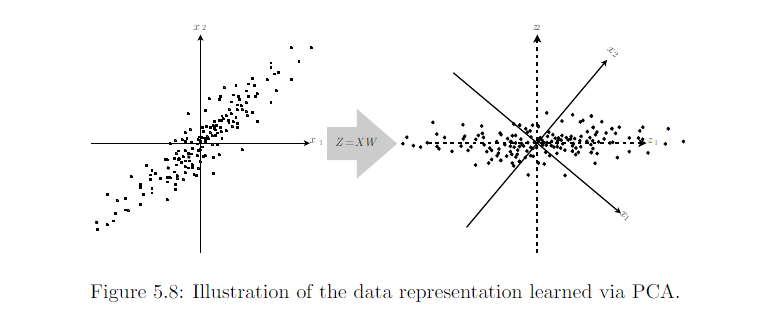
PCA is an orthogonal, linear transformation of the data that projects it into a representation where the elements are uncorrelated.



We can use PCA as a simple and effective dimensionality reduction method that preserves as much of the information in the data as possible (measured by least-squares reconstruction error).

Let us consider the n×m-dimensional design matrix X.

The data has a mean of zero, E[x]=0

The unbiased sample covariance matrix is given by: Var[x]=1n−1XTX

PCA finds a representation (through linear transformation) z=Wx where Var[z] is diagonal. To do this, we will make use of the singular value decomposition (SVD) of X: X=UΣWT,.

where Σ is an n×m-dimensional rectangular diagonal matrix with the singular values of X on the main diagonal, UU is an n×nn×n matrix whose columns are orthonormal (i.e. unit length and orthogonal) and WW is an m ×mm×m matrix also composed of orthonormal column vectors.

Var[x]=1n−1XTX=1n−1WΣ2WT

Var[z]=1n−1ZTZ=1n−1WTXTXW=1n−1WWTΣ2WWT=1n−1Σ2

The individual elements of z are mutually uncorrelated.

In the case of PCA, this disentangling takes the form of finding a rotation of the input space (mediated via the transformation W ) that aligns the principal axes of variance with the basis of the new representation space associated with z,

Weakly Supervised Learning

It refers to a setting where the datasets consists of (x,y) pairs, as in supervised learning, but where the labels y are either unreliably present (i.e. with missing values) or noisy (i.e. where the label given is not the true label).

Building a Machine Learning Algorithm

Nearly all deep learning algorithms can be described as particular instances of a fairly simple recipe: combine a specification of a dataset, a cost function, an optimization procedure and a model.

For example, the linear regression algorithm:

dataset consists of X and y

cost function:J(w,b)=−Ex,y∼p^datapmodel(y∣x)

model: pmodel(y∣x)=N(y∣xTw+b,1)

optimization: gradient descent, stochastic gradient descent or SGD