residuals gam

In many social science and business problems, it is often more important to explain why a phenomenon happens than improving the model’s predictability on the event happening. Having an interpretable model is, therefore, crucial in understanding how different factors interact with the outcome of interest.

在许多社会科学和商业问题中，解释现象为什么会比提高事件发生时模型的可预测性通常更重要。 因此，拥有一个可解释的模型对于理解不同因素如何与感兴趣的结果相互作用至关重要。

The model’s interpretability is also important in highly regulated business environments, such as loan approval decisions. Even in situations where prediction accuracy is more important than the “why”, an interpretable model can help debug more complicated models and guide new approaches to feature engineering and data preprocessing.

该模型的可解释性在高度监管的业务环境(例如贷款批准决策)中也很重要。 即使在预测精度比“为什么”更为重要的情况下，可解释的模型也可以帮助调试更复杂的模型，并指导特征工程和数据预处理的新方法。

GAM-引擎盖下 (GAM — under the hood)

In this context, generalized additive models (GAM) offer a middle ground between simple models, such as those we fit with linear regression, and more sophisticated machine learning models like neural networks that usually promise superior prediction performance to simple models. GAM can also be used in various tasks: regression, classification, binary choice.

在这种情况下，广义加性模型(GAM)在简单模型(例如我们适合线性回归的模型)和更复杂的机器学习模型(例如神经网络)之间提供了中间立场，这些模型通常比简单模型具有更好的预测性能。 GAM还可以用于各种任务：回归，分类，二元选择。

In linear regression, we model outcome y as a function of 2 inputs X₁ and X₂ with the following:

在线性回归中，我们将结果y建模为2个输入X 1和X 2的函数，其结果如下：

y = β₁X₁ + β₂ X₂ + u

y =β₁X₁+β2X2 + u

In GAM, the β Xᵢ is replaced by f(Xᵢ), where f() can be any arbitrary nonlinear functions. In other words, GAM is composed of a sum of smooth functions f() on the input. The idea is still that each input feature makes a separate contribution to the response, and these just add up, but these contributions don’t have to be strictly proportional to the inputs. The beauty of this approach is that, similar to what β represents in linear regression, the partial response function f() still captures the change on outcome y to change the input. The change in prediction depends on the initial value of Xᵢ.

在GAM中，βXᵢ被f(Xᵢ)代替，其中f()可以是任意非线性函数。 换句话说，GAM由输入上的平滑函数f()的总和组成。 想法仍然是，每个输入要素都对响应做出单独的贡献，这些只是相加而已，但是这些贡献不必严格地与输入成比例。 这种方法的优点在于，类似于β在线性回归中表示的那样，部分响应函数f()仍捕获结果y的变化以更改输入。 预测的变化取决于Xᵢ的初始值。

A common approach to deal with nonlinear relationships in regression models involves creating polynomial features. For the predictor in question, Xᵢ, we add terms e.g. quadratic (Xᵢ²), cubic (Xᵢ³), etc to get a better fit. GAM encompasses this idea but includes an additional aspect: penalized estimation. The idea is similar to that of a ridge or lasso regression, where penalty terms are added to help avoid overfitting.

处理回归模型中非线性关系的常用方法包括创建多项式特征。 对于有问题的预测变量Xᵢ，我们添加了二次项(Xquad²)，三次方(Xᵢ³)等项，以获得更好的拟合度。 GAM包含了这个想法，但还包括一个附加方面： 惩罚性估算 。 这个想法类似于ridge或lasso回归的想法，其中添加了惩罚项以帮助避免过拟合。

Another way of creating transformations of a variable is to cut the variable into distinct regions, and fit those regions separately. However, the different fits could be unconnected, leading to sometimes notably different predictions for values close together. GAM allows the user to specify the number of

knots

in the variable, which are used to create sections where separate cubic polynomials are fit at each section and then joined to create a continuous curve.

创建变量转换的另一种方法是将变量切成不同的区域，然后分别拟合这些区域。 但是，不同的拟合可能是不相关的，有时会导致对值相互靠近的明显不同的预测。 GAM允许用户在变量中指定

knots

数，这些

knots

数用于创建节，在

knots

中将单独的三次多项式拟合到每个节，然后将其合并以创建连续曲线。

那么应该使用什么平滑函数？ (So what smooth function should be used?)

A number of smooths are available with the mgcv package in R, and one can learn more via the help file for smooth.terms (link). The default is thin plate regression splines (TPRS), which works well in general in terms of performance. Cubic spline is also a common basis that mirrors adding polynomial terms for the covariates.

R中的mgcv软件包提供了许多平滑器，并且可以通过帮助文件获取有关smooth.terms ( 链接 )的更多信息。 默认设置为薄板回归样条(TPRS)，通常在性能方面效果很好。 三次样条也是映射共变量的多项式项的常见基础。

在R中实施 (Implementing in R)

We use the

mgcv

package in `R` to implement gam and use a built-in dataset

medcare

from the package

catdata

to illustrate gam and compare with the performance using logistic regression.

我们使用

mgcv

包`R`实施GAM并使用内置的数据集

medcare

从包装

catdata

来说明GAM和使用logistic回归的性能进行比较。

The

medcare

data was collected on 4406 individuals, aged 66 and over, that were covered by a public insurance program. The outcome variable is

healthpoor

, a binary variable that equals 1 if the individual reports poor health and 0 otherwise. We are interested in knowing how

ofp

, the number of physician office visits, might be correlated with health outcomes. One can hypothesize a nonlinear relationship between the two variables: a healthy individual will have few physician visits, but having more visits also allow the patients to return to be more healthy. So we are interested to have a more flexible modeling approach.

medcare

数据收集了4406名66岁及以上的个人，这些人已获得公共保险计划的覆盖。 结果变量是

healthpoor

，如果个人报告的健康状况不佳，则该二进制变量等于1，否则为0。 我们感兴趣的是知道如何

ofp

，医生办公室访问的次数，可能与健康状况有关。 一个人可以假设这两个变量之间存在非线性关系：一个健康的人很少去看医生，但是去更多的人也可以使病人恢复健康。 因此，我们有兴趣提供一种更加灵活的建模方法。

The mgcv treats

gam

as a generalized version of

glm

, so one can directly call the

gam

method to use

glm

methods such as linear and logistic regression.

mgcv将

gam

视为

glm

的广义版本，因此可以直接调用

gam

方法来使用

glm

方法，例如线性和逻辑回归。

library(catdata)
library(mgcv)
library(Metrics)
library(ggplot2)
library(visreg)data(medcare)#### logit model (same as running glm with family set to "binomial")
lm <- gam(healthpoor ~ male+ age + ofp, family = binomial, data = medcare)
pred <- predict(lm, type="response")
lm_auc <- Metrics::auc(medcare$healthpoor, pred)
lm_auc#### generalized additive model
gam <- gam(healthpoor ~ male+s(age)+s(ofp), family = binomial, data = medcare)
pred <- predict(gam, type="response")
gam_auc <- Metrics::auc(medcare$healthpoor, pred)
gam_auc

The s() terms in the gam formula indicate which terms are to be smoothed. There are several options you can pass on to the s() terms — for example, you can specify a different smooth function

bs

, and a different number of knots

k

.

gam公式中的s()项指示要平滑的项。 可以将s()项传递给多个选项-例如，可以指定不同的平滑函数

bs

和不同的结

k

。

If the number of unique values is less than the number of basis (For example, when you tried to add

s()

to a binary variable like

male

), the function would return the following error:

如果唯一值的数量小于基数(例如，当您尝试将

s()

添加到类似于

male

的二进制变量时)，该函数将返回以下错误：

A term has fewer unique covariate combinations than specified maximum degrees of freedom.

一个术语的唯一协变量组合少于指定的最大自由度。

Using

visreg

to visualize the fitted terms of

ofp

, we can see that

gam

produces a much more nuanced prediction of

ofp

while that of the logistic regression is much more linear.

使用

visreg

可视化的拟合方面

ofp

，我们可以看到，

gam

产生的微妙得多预测

ofp

而Logistic回归的更加线性。

visreg(gam, "ofp", jitter=TRUE, line=list(col="red"),
       fill=list(col="green"))

The

gam

model also yields a slightly better AUC, 0.679, versus 0.673 of the logistic regression.

gam

模型还产生了更好的AUC(0.679)，而logistic回归为0.673。

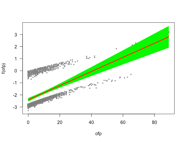IPrediction based on ofp: gam (left), logistic regression (right). mage by Author. 基于ofp的IP预测：gam(左)，逻辑回归(右)。 作者的法师。

解释 (Interpretation)

We are ultimately interested in estimating the change in

ofp

on the probability of

healthpoor

. To do that, we need to fix the other features’ values to their mean or mode(if the feature is a categorical variable). We then create a test dataframe that has a list of possible values of

ofp

.

我们最终希望评估的变化

ofp

上的概率

healthpoor

。 为此，我们需要将其他特征的值固定为其平均值或众数(如果特征是分类变量)。 然后，我们创建一个测试数据框，其中包含可能的

ofp

值列表。

# function to get mode of an array of values
getmode <- function(v) {
  uniqv <- unique(v)
  uniqv[which.max(tabulate(match(v, uniqv)))]
}testdata = data.frame(ofp = seq(0, 100, length = 101),
                      male = getmode(gam$model$male),
                      age = mean(gam$model$age))

Using the

predict

function, we can then extrapolate the previously fitted gam model to the test data. The plot shows that

ofp

has a nonlinear relationship with the likelihood of reporting poor health, holding other variables constant. Furthermore, the confidence interval less tight in regions with higher ofp.

然后，使用

predict

功能，我们可以将先前拟合的gam模型外推到测试数据。 该图显示，

ofp

与报告不良健康状况的可能性具有非线性关系，而其他变量不变。 此外，置信区间在具有较高ofp的区域中不那么紧密。

fits = predict(gam, newdata=testdata, type='response', se=T)### create a confidence interval for the fits
predicts = data.frame(testdata, fits) %>% 
  mutate(lower = fit - 1.96*se.fit,
         upper = fit + 1.96*se.fit)ggplot(aes(x=ofp,y=fit), data=predicts) +
  geom_ribbon(aes(ymin = lower, ymax=upper), fill='gray90') +
  geom_line(color='#00aaff') +theme_bw()

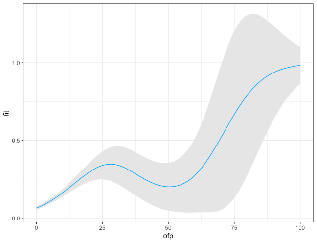Image by Author. 图片由作者提供。

翻译自: https://towardsdatascience.com/gam-a-flexible-modeling-approach-that-preserves-interpretability-a68a4f235b6e

residuals gam