This paper shows how Long Short-term Memory recurrent neural net- works can be used to generate complex sequences with long-range struc- ture, simply by predicting one data point at a time. The approach is demonstrated for text (where the data are discrete) and online handwrit- ing (where the data are real-valued). It is then extended to handwriting synthesis by allowing the network to condition its predictions on a text sequence. The resulting system is able to generate highly realistic cursive handwriting in a wide variety of styles.

利用短期记忆递归神经网络，通过简单地预测一个数据点来实现长时间的复杂序列生成。该方法适用于文本(数据是离散的)和在线手写(数据是实值的)。然后，通过允许网络根据文本序列调整预测，将其扩展到手写合成。由此产生的系统能够生成多种风格的高度逼真的草书。

1、Introduction

Recurrent neural networks (RNNs) are a rich class of dynamic models that have been used to generate sequences in domains as diverse as music [6, 4], text [30] and motion capture data [29]. RNNs can be trained for sequence generation by processing real data sequences one step at a time and predicting what comes next. Assuming the predictions are probabilistic, novel sequences can be gener- ated from a trained network by iteratively sampling from the network’s output distribution, then feeding in the sample as input at the next step. In other words by making the network treat its inventions as if they were real, much like a person dreaming. Although the network itself is deterministic, the stochas- ticity injected by picking samples induces a distribution over sequences. This distribution is conditional, since the internal state of the network, and hence its predictive distribution, depends on the previous inputs.	1、介绍递归神经网络(RNNs)是一类丰富的动态模型，被用于生成音乐[6,4]、文本[30]和动作捕捉数据[29]等领域的序列。通过一步一步地处理真实的数据序列并预测接下来会发生什么，可以训练RNNs来生成序列。假设预测是概率性的，通过对网络的输出分布进行迭代采样，然后将样本作为下一步的输入，可以从训练好的网络中生成新的序列。换句话说，通过让网络把它的发明当作是真实的，就像一个人在做梦一样。虽然网络本身是确定性的，但通过取样注入的随机度会导致序列上的分布。这种分布是有条件的，因为网络的内部状态(因此它的预测分布)取决于以前的输入。
RNNs are ‘fuzzy’ in the sense that they do not use exact templates from the training data to make predictions, but rather—like other neural networks— use their internal representation to perform a high-dimensional interpolation between training examples. This distinguishes them from n-gram models and compression algorithms such as Prediction by Partial Matching [5], whose pre- dictive distributions are determined by counting exact matches between the recent history and the training set. The result—which is immediately appar- ent from the samples in this paper—is that RNNs (unlike template-based al- gorithms) synthesise and reconstitute the training data in a complex way, and rarely generate the same thing twice. Furthermore, fuzzy predictions do not suf- fer from the curse of dimensionality, and are therefore much better at modelling real-valued or multivariate data than exact matches.	从某种意义上说，RNNs是“模糊的”，因为它们不使用来自训练数据的准确模板来进行预测，而是像其他神经网络一样，使用它们的内部表示来在训练实例之间执行高维插值。这将它们与n-gram模型和压缩算法(如通过部分匹配[5]进行预测)进行了区分，后者的预测分布是通过计算最近历史与训练集之间的精确匹配来确定的从本文的样本中可以看出，RNNs(与基于模板的算法不同)以一种复杂的方式综合和重构训练数据，并且很少生成相同的内容两次。此外，模糊预测不依赖于维数的诅咒，因此在建模实值或多变量数据时，它比精确匹配要有效得多。
In principle a large enough RNN should be sufficient to generate sequences of arbitrary complexity. In practice however, standard RNNs are unable to store information about past inputs for very long [15]. As well as diminishing their ability to model long-range structure, this ‘amnesia’ makes them prone to instability when generating sequences. The problem (common to all conditional generative models) is that if the network’s predictions are only based on the last few inputs, and these inputs were themselves predicted by the network, it has little opportunity to recover from past mistakes. Having a longer memory has a stabilising effect, because even if the network cannot make sense of its recent history, it can look further back in the past to formulate its predictions. The problem of instability is especially acute with real-valued data, where it is easy for the predictions to stray from the manifold on which the training data lies. One remedy that has been proposed for conditional models is to inject noise into the predictions before feeding them back into the model [31], thereby increasing the model’s robustness to surprising inputs. However we believe that a better memory is a more profound and effective solution.	原则上，一个足够大的RNN应该足以生成任意复杂度的序列。然而，在实践中，标准的rns不能存储关于非常长的[15]的过去输入的信息。这种“健忘症”不仅会削弱他们对长期结构建模的能力，还会使他们在生成序列时变得不稳定。问题是(所有条件生成模型共有的)，如果网络的预测仅仅基于最后的几个输入，而这些输入本身是由网络预测的，那么它几乎没有机会从过去的错误中恢复过来。拥有更长的记忆有一个稳定的效果，因为即使网络不能理解它最近的历史，它可以回顾过去来制定它的预测。对于实值数据来说，不稳定性问题尤其严重，因为预测很容易偏离训练数据所在的流形。针对条件模型提出的一个补救措施是，在将预测反馈回模型[31]之前，在预测中加入噪音，从而提高模型对意外输入的鲁棒性。然而，我们相信更好的记忆是一个更深刻和有效的解决方案。
Long Short-term Memory (LSTM) [16] is an RNN architecture designed to be better at storing and accessing information than standard RNNs. LSTM has recently given state-of-the-art results in a variety of sequence processing tasks, including speech and handwriting recognition [10, 12]. The main goal of this paper is to demonstrate that LSTM can use its memory to generate complex, realistic sequences containing long-range structure.	长短时记忆(LSTM)[16]是一种RNN结构，它比标准的rns更适合于存储和访问信息。LSTM最近在一系列序列处理任务中给出了最先进的结果，包括语音和手写识别[10,12]。本文的主要目的是证明LSTM可以利用它的内存来生成复杂的、真实的、包含长程结构的序列。
Figure 1: Deep recurrent neural network prediction architecture. The circles represent network layers, the solid lines represent weighted connections and the dashed lines represent predictions.	图1:深度递归神经网络预测体系结构。圆圈表示网络层，实线表示加权连接，虚线表示预测。
Section 2 defines a ‘deep’ RNN composed of stacked LSTM layers, and ex- plains how it can be trained for next-step prediction and hence sequence gener- ation. Section 3 applies the prediction network to text from the Penn Treebank and Hutter Prize Wikipedia datasets. The network’s performance is compet- itive with state-of-the-art language models, and it works almost as well when predicting one character at a time as when predicting one word at a time. The highlight of the section is a generated sample of Wikipedia text, which showcases the network’s ability to model long-range dependencies. Section 4 demonstrates how the prediction network can be applied to real-valued data through the use of a mixture density output layer, and provides experimental results on the IAM Online Handwriting Database. It also presents generated handwriting samples proving the network’s ability to learn letters and short words direct from pen traces, and to model global features of handwriting style. Section 5 introduces an extension to the prediction network that allows it to condition its outputs on a short annotation sequence whose alignment with the predictions is unknown. This makes it suitable for handwriting synthesis, where a human user inputs a text and the algorithm generates a handwritten version of it. The synthesis network is trained on the IAM database, then used to generate cursive hand- writing samples, some of which cannot be distinguished from real data by the naked eye. A method for biasing the samples towards higher probability (and greater legibility) is described, along with a technique for ‘priming’ the samples on real data and thereby mimicking a particular writer’s style. Finally, concluding remarks and directions for future work are given in Section 6.	第2节定义了一个由多层LSTM层组成的“深度”RNN，并讨论了如何训练它来进行下一步预测，从而实现序列生成。第3节将预测网络应用于来自Penn Treebank和Hutter Prize Wikipedia数据集的文本。该网络的性能与最先进的语言模型是竞争的，它在预测一个字符时的效果几乎与预测一个单词时的效果一样好。本节的重点是生成的Wikipedia文本样本，它展示了网络建模长期依赖项的能力。第4节演示了如何通过混合密度输出层将预测网络应用于实值数据，并提供了IAM在线手写数据库的实验结果。它还提供了生成的手写样本，证明该网络能够直接从手写轨迹学习字母和短单词，并对手写风格的全局特征进行建模。第5节介绍了对预测网络的扩展，该扩展允许预测网络将其输出设置为与预测一致的短注释序列。这使得它适用于手写合成，即人类用户输入文本，然后算法生成手写版本。综合网络在IAM数据库上进行训练，然后生成草书手写样本，其中一些无法用肉眼分辨出真实数据。描述了一种将样本偏向于更高概率(以及更大的易读性)的方法，以及一种在真实数据上“启动”样本从而模仿特定作者风格的技术。最后，第六节给出结论和今后工作的方向。

2 Prediction Network 预测网络

Fig. 1 illustrates the basic recurrent neural network prediction architecture used in this paper. An input vector sequence x = (x1, . . . , xT ) is passed through weighted connections to a stack of N recurrently connected hidden layers to compute first the hidden vector sequences h n = (h n 1 , . . . , hn T ) and then the output vector sequence y = (y1, . . . , yT ). Each output vector yt is used to parameterise a predictive distribution Pr(xt+1|yt) over the possible next inputs xt+1. The first element x1 of every input sequence is always a null vector whose entries are all zero; the network therefore emits a prediction for x2, the first real input, with no prior information. The network is ‘deep’ in both space and time, in the sense that every piece of information passing either vertically or horizontally through the computation graph will be acted on by multiple successive weight matrices and nonlinearities.

图1给出了本文所采用的基本递归神经网络预测体系结构。一个输入向量序列x = (x1，…， xT)通过加权连接到N个递归连接的隐层堆栈中，首先计算隐藏向量序列h N = (h N 1，…然后输出向量序列y = (y1，…次)。每个输出向量yt被用来参数化一个预测分布Pr(xt+1|yt)对可能的下一个输入xt+1。每个输入序列的第一个元素x1总是一个零向量，它的所有元素都是零;因此，该网络发出对x2的预测，x2是第一个实际输入，没有先验信息。这个网络在空间和时间上都是“深”的，也就是说，通过计算图垂直或水平传递的每一条信息都将受到多个连续的权重矩阵和非线性的影响。

Note the ‘skip connections’ from the inputs to all hidden layers, and from all hidden layers to the outputs. These make it easier to train deep networks, by reducing the number of processing steps between the bottom of the network and the top, and thereby mitigating the ‘vanishing gradient’ problem [1]. In the special case that N = 1 the architecture reduces to an ordinary, single layer next step prediction RNN.

注意从输入到所有隐藏层的“跳过连接”，以及从所有隐藏层到输出的“跳过连接”。通过减少网络底部和顶部之间的处理步骤的数量，从而降低了训练深度网络的难度，从而减轻了[1]的“消失梯度”问题。在N = 1的特殊情况下，该体系结构简化为一个普通的单层下一步预测RNN。

The hidden layer activations are computed by iterating the following equations from t = 1 to T and from n = 2 to N

where the W terms denote weight matrices (e.g. Wihn is the weight matrix connecting the inputs to the n th hidden layer, Wh1h1 is the recurrent connection at the first hidden layer, and so on), the b terms denote bias vectors (e.g. by is output bias vector) and H is the hidden layer function.

Given the hidden sequences, the output sequence is computed as follow:

where Y is the output layer function. The complete network therefore defines a function, parameterised by the weight matrices, from input histories x1:t to output vectors yt.

The output vectors yt are used to parameterise the predictive distribution Pr(xt+1|yt) for the next input. The form of Pr(xt+1|yt) must be chosen carefully to match the input data. In particular, finding a good predictive distribution for high-dimensional, real-valued data (usually referred to as density modelling), can be very challenging.

The probability given by the network to the input sequence x

The partial derivatives of the loss with respect to the network weights can be efficiently calculated with backpropagation through time [33] applied to the computation graph shown in Fig. 1, and the network can then be trained with gradient descen

隐层激活的计算方法如下:从t = 1到t，从n = 2到n

矩阵W术语表示的重量(例如Wihn权重矩阵连接输入n th隐藏层,Wh1h1是复发性连接在第一个隐藏层,等等),b项表示偏差向量(例如输出偏差向量)和H是隐藏层的功能。

给定隐藏序列，输出序列计算如下:

其中Y为输出层函数。因此，整个网络定义了一个函数，由权矩阵参数化，从输入历史x1:t到输出向量yt。

输出向量yt用于参数化下一个输入的预测分布Pr(xt+1|yt)。必须仔细选择Pr(xt+1|yt)的形式来匹配输入数据。特别是，为高维、实值数据(通常称为密度建模)找到一个好的预测分布是非常具有挑战性的。

由网络给出的输入序列x的概率

通过对图1所示的计算图进行时间[33]的反向传播，可以有效地计算出损失相对于网络权值的偏导数，然后通过梯度下行对网络进行训练

2.1 Long Short-Term Memory

Figure 2: Long Short-term Memory Cell

In most RNNs the hidden layer function H is an elementwise application of a sigmoid function. However we have found that the Long Short-Term rm Memory (LSTM) architecture [16], which uses purpose-built memory cells to store information, is better at finding and exploiting long range dependencies in the data. Fig. 2 illustrates a single LSTM memory cell. For the version of LSTM used in this paper [7] H is implemented by the following composite function:

where σ is the logistic sigmoid function, and i, f, o and c are respectively the input gate, forget gate, output gate, cell and cell input activation vectors, all of which are the same size as the hidden vector h. The weight matrix subscripts have the obvious meaning, for example Whi is the hidden-input gate matrix, Wxo is the input-output gate matrix etc. The weight matrices from the cell to gate vectors (e.g. Wci) are diagonal, so element m in each gate vector only receives input from element m of the cell vector. The bias terms (which are added to i, f, c and o) have been omitted for clarity.

图2:长短时记忆细胞

在大多数网络中，隐层函数H是s型函数的基本应用。然而，我们发现，使用专门构建的内存单元来存储信息的长短期rm内存(LSTM)体系结构[16]更善于发现和利用数据中的长期依赖关系。图2显示了单个LSTM存储单元。对于本文使用的LSTM版本，[7]H通过以下复合函数实现:

σ是物流乙状结肠函数,和我,f, o和c分别输入门,忘记门,输出门,细胞和细胞激活输入向量,都是同样的大小隐藏向量h。权重矩阵下标有明显的意义,例如Whi隐藏输入门矩阵,Wxo输入-输出门矩阵等。单元到栅极向量(如Wci)的权重矩阵是对角的，因此每个栅极向量中的m元素只接收单元向量的m元素的输入。偏置项(添加到i、f、c和o中)被省略，以保持清晰。

The original LSTM algorithm used a custom designed approximate gradient calculation that allowed the weights to be updated after every timestep [16]. However the full gradient can instead be calculated with backpropagation through time [11], the method used in this paper. One difficulty when training LSTM with the full gradient is that the derivatives sometimes become excessively large,leading to numerical problems. To prevent this, all the experiments in this paper clipped the derivative of the loss with respect to the network inputs to the LSTM layers (before the sigmoid and tanh functions are applied) to lie within a predefined range1 .

原始的LSTM算法使用了自定义设计的近似梯度计算，允许在每一步[16]之后更新权值。然而，全梯度可以通过时间[11]的反向传播来计算，这是本文使用的方法。用全梯度法训练LSTM的一个难点是导数有时会变得过大，导致数值问题。为了防止这种情况，本文中的所有实验都将损耗对LSTM层的网络输入的导数(在应用sigmoid和tanh函数之前)限制在预定义的范围e1内。

3 Text Prediction 文本预测

Text data is discrete, and is typically presented to neural networks using ‘onehot’ input vectors. That is, if there are K text classes in total, and class k is fed in at time t, then xt is a length K vector whose entries are all zero except for the k th, which is one. Pr(xt+1|yt) is therefore a multinomial distribution, which can be naturally parameterised by a softmax function at the output layer:

文本数据是离散的，通常使用“onehot”输入向量呈现给神经网络。也就是说，如果总共有K个文本类，而类K是在t时刻输入的，那么xt就是一个长度为K的向量，除了第K项是1外，其他项都是0。因此，Pr(xt+1|yt)是一个多项分布，可以通过输出层的softmax函数自然参数化:

The only thing that remains to be decided is which set of classes to use. In most cases, text prediction (usually referred to as language modelling) is performed at the word level. K is therefore the number of words in the dictionary. This can be problematic for realistic tasks, where the number of words (including variant conjugations, proper names, etc.) often exceeds 100,000. As well as requiring many parameters to model, having so many classes demands a huge amount of training data to adequately cover the possible contexts for the words. In the case of softmax models, a further difficulty is the high computational cost of evaluating all the exponentials during training (although several methods have been to devised make training large softmax layers more efficient, including tree-based models [25, 23], low rank approximations [27] and stochastic derivatives [26]). Furthermore, word-level models are not applicable to text data containing non-word strings, such as multi-digit numbers or web addresse.

唯一需要决定的是使用哪一组类。在大多数情况下，文本预测(通常称为语言建模)是在单词级执行的。因此K是字典中的单词数。这对于实际的任务来说是有问题的，因为单词的数量(包括不同的词形变化、专有名称等)常常超过100,000。除了需要许多参数进行建模外，拥有如此多的类还需要大量的训练数据来充分覆盖单词的可能上下文。在softmax模型中，另一个困难是在训练期间评估所有指数的计算成本很高(尽管已经设计了几种方法来提高训练大型softmax层的效率，包括基于树的模型[25,23]、低秩近似[27]和随机导数[26])。此外，单词级模型不适用于包含非单词字符串的文本数据，如多位数字或web地址。

Character-level language modelling with neural networks has recently been considered [30, 24], and found to give slightly worse performance than equivalent word-level models. Nonetheless, predicting one character at a time is more interesting from the perspective of sequence generation, because it allows the network to invent novel words and strings. In general, the experiments in this paper aim to predict at the finest granularity found in the data, so as to maximise the generative flexibility of the networ

使用神经网络的字符级语言建模最近被考虑[30,24]，并发现其性能略差于等价的字级模型。尽管如此，从序列生成的角度来看，一次预测一个字符更有趣，因为它允许网络创建新的单词和字符串。总的来说，本文的实验旨在以数据中发现的最细粒度进行预测，从而最大限度地提高网络的生成灵活性

3.1 Penn Treebank Experiments Penn Treebank实验

The first set of text prediction experiments focused on the Penn Treebank portion of the Wall Street Journal corpus [22]. This was a preliminary study whose main purpose was to gauge the predictive power of the network, rather than to generate interesting sequences.	第一组文本预测实验集中在《华尔街日报》语料库[22]的宾夕法尼亚河岸部分。这是一项初步研究，其主要目的是评估网络的预测能力，而不是生成有趣的序列。
Although a relatively small text corpus (a little over a million words in total), the Penn Treebank data is widely used as a language modelling benchmark. The training set contains 930,000 words, the validation set contains 74,000 words and the test set contains 82,000 words. The vocabulary is limited to 10,000 words, with all other words mapped to a special ‘unknown word’ token. The end-ofsentence token was included in the input sequences, and was counted in the sequence loss. The start-of-sentence marker was ignored, because its role is already fulfilled by the null vectors that begin the sequences (c.f. Section 2).	尽管文本语料库相对较小(总共超过100万单词)，Penn Treebank的数据被广泛用作语言建模的基准。训练集包含93万字，验证集包含7.4万字，测试集包含8.2万字。词汇表被限制为10,000个单词，所有其他单词都映射到一个特殊的“未知单词”标记。语句结束标记被包含在输入序列中，并被计算在序列丢失中。句子开始标记被忽略，因为它的作用已经由开始序列的空向量完成(c.f. . Section 2)。
The experiments compared the performance of word and character-level LSTM predictors on the Penn corpus. In both cases, the network architecture was a single hidden layer with 1000 LSTM units. For the character-level network the input and output layers were size 49, giving approximately 4.3M weights in total, while the word-level network had 10,000 inputs and outputs and around 54M weights. The comparison is therefore somewhat unfair, as the word-level network had many more parameters. However, as the dataset is small, both networks were easily able to overfit the training data, and it is not clear whether the character-level network would have benefited from more weights. All networks were trained with stochastic gradient descent, using a learn rate of 0.0001 and a momentum of 0.99. The LSTM derivates were clipped in the range [−1, 1] (c.f. Section 2.1).	实验比较了词级和字符级LSTM预测器在Penn语料库上的性能。在这两种情况下，网络架构都是一个包含1000 LSTM单元的单一隐含层。对于字符级网络，输入和输出层的大小为49，总共给出了大约430万的权重，而单词级网络有10,000个输入和输出，以及大约54M的权重。因此，这种比较有点不公平，因为单词级网络有更多的参数。然而，由于数据集较小，这两个网络都很容易对训练数据进行过度拟合，而且还不清楚字符级网络是否会从更大的权重中受益。所有网络均采用随机梯度下降训练，学习率为0.0001，动量为0.99。LSTM衍生物被限制在[−1,1]范围内(c.f。2.1节)。
Neural networks are usually evaluated on test data with fixed weights. For prediction problems however, where the inputs are the targets, it is legitimate to allow the network to adapt its weights as it is being evaluated (so long as it only sees the test data once). Mikolov refers to this as dynamic evaluation. Dynamic evaluation allows for a fairer comparison with compression algorithms, for which there is no division between training and test sets, as all data is only predicted once.	神经网络的评价通常采用固定权值的试验数据。然而，对于输入是目标的预测问题，允许网络在评估时调整其权重是合理的(只要它只看到测试数据一次)。Mikolov称之为动态评估。动态评估允许与压缩算法进行更公平的比较，压缩算法不需要划分训练集和测试集，因为所有数据只预测一次。
Table 1: Penn Treebank Test Set Results. ‘BPC’ is bits-per-character. ‘Error’ is next-step classification error rate, for either characters or words.	表1:Penn Treebank测试集的结果。BPC的bits-per-character。“错误”是下一步的分类错误率，不管是字符还是单词。
Since both networks overfit the training data, we also experiment with two types of regularisation: weight noise [18] with a std. deviation of 0.075 applied to the network weights at the start of each training sequence, and adaptive weight noise [8], where the variance of the noise is learned along with the weights using a Minimum description Length (or equivalently, variational inference) loss function. When weight noise was used, the network was initialised with the final weights of the unregularised network. Similarly, when adaptive weight noise was used, the weights were initialised with those of the network trained with weight noise. We have found that retraining with iteratively increased regularisation is considerably faster than training from random weights with regularisation. Adaptive weight noise was found to be prohibitively slow for the word-level network, so it was regularised with fixed-variance weight noise only. One advantage of adaptive weight is that early stopping is not needed (the network can safely be stopped at the point of minimum total ‘description length’ on the training data). However, to keep the comparison fair, the same training, validation and test sets were used for all experiments.	因为网络overfit训练数据,我们也尝试两种regularisation:体重噪声[18]std.偏差为0.075应用于网络权值在每个训练序列的开始,体重和自适应噪声[8],噪声的方差在哪里学习使用最小描述长度随着重量损失函数(或等价变分推理)。当使用权值噪声时，网络被初始化为非正则化网络的最终权值。类似地，当使用自适应权值噪声时，权值与使用权值噪声训练的网络的权值初始化。我们发现，用迭代增加的正则化进行再训练要比用正则化进行随机加权训练快得多。自适应权值噪声在词级网络中速度非常慢，因此只能用固定方差权值噪声对其进行正则化。自适应权值的一个优点是不需要提前停止(网络可以安全地在训练数据上的最小总“描述长度”处停止)。然而，为了保持比较的公平性，所有的实验都使用相同的训练、验证和测试集。
The results are presented with two equivalent metrics: bits-per-character (BPC), which is the average value of − log2 Pr(xt+1\|yt) over the whole test set; and perplexity which is two to the power of the average number of bits per word (the average word length on the test set is about 5.6 characters, so perplexity ≈ 2 5.6BP C ). Perplexity is the usual performance measure for language modelling.	结果用两个等价的度量来表示:每个字符的比特数(BPC)，这是−log2 Pr(xt+1\|yt)在整个测试集上的平均值;perplexity为每个单词平均位数的2次方(测试集上的平均单词长度约为5.6个字符，所以perplexity≈2 5.6 bp C)。Perplexity是语言建模的常用性能度量。
Table 1 shows that the word-level RNN performed better than the characterlevel network, but the gap appeared to close when regularisation is used. Overall the results compare favourably with those collected in Tomas Mikolov’s thesis [23]. For example, he records a perplexity of 141 for a 5-gram with KeyserNey smoothing, 141.8 for a word level feedforward neural network, 131.1 for the state-of-the-art compression algorithm PAQ8 and 123.2 for a dynamically evaluated word-level RNN. However by combining multiple RNNs, a 5-gram and a cache model in an ensemble, he was able to achieve a perplexity of 89.4. Interestingly, the benefit of dynamic evaluation was far more pronounced here than in Mikolov’s thesis (he records a perplexity improvement from 124.7 to 123.2 with word-level RNNs). This suggests that LSTM is better at rapidly adapting to new data than ordinary RNNs.	表1显示，单词级RNN的性能优于字符级网络，但在使用正则化时，这种差距似乎缩小了。总的来说，这些结果与Tomas Mikolov的论文[23]中收集到的结果相比是令人满意的。例如，他记录了5克KeyserNey平滑算法的perplexity为141，单词级前馈神经网络的perplexity为141.8，最先进的压缩算法PAQ8的perplexity为131.1，动态评估单词级RNN的perplexity为123.2。然而，通过将多个RNNs、一个5克重的内存和一个缓存模型结合在一起，他可以得到一个令人困惑的89.4。有趣的是，动态评估的好处在这里比在Mikolov的论文中更明显(他记录了一个复杂的改进，从124.7到123.2的单词级RNNs)。这表明LSTM在快速适应新数据方面优于普通的rns。

3.2 Wikipedia Experiments 维基百科的实验

In 2006 Marcus Hutter, Jim Bowery and Matt Mahoney organised the following challenge, commonly known as Hutter prize [17]: to compress the first 100 million bytes of the complete English Wikipedia data (as it was at a certain time on March 3rd 2006) to as small a file as possible. The file had to include not only the compressed data, but also the code implementing the compression algorithm. Its size can therefore be considered a measure of the minimum description length [13] of the data using a two part coding scheme.	在2006年，Marcus Hutter, Jim Bowery和Matt Mahoney组织了如下的挑战，通常被称为Hutter奖[17]:压缩完整的英文维基百科数据的前1亿字节(在2006年3月3日的某个时间)到一个尽可能小的文件。该文件不仅要包含压缩数据，还要包含实现压缩算法的代码。因此，它的大小可以被认为是使用两部分编码方案的数据的最小描述长度[13]的度量。
Wikipedia data is interesting from a sequence generation perspective because it contains not only a huge range of dictionary words, but also many character sequences that would not be included in text corpora traditionally used for language modelling. For example foreign words (including letters from nonLatin alphabets such as Arabic and Chinese), indented XML tags used to define meta-data, website addresses, and markup used to indicate page formatting such as headings, bullet points etc. An extract from the Hutter prize dataset is shown in Figs. 3 and 4.	从序列生成的角度来看，Wikipedia的数据非常有趣，因为它不仅包含大量的字典单词，而且还包含许多字符序列，而这些字符序列不会包含在传统用于语言建模的文本语料库中。例如，外来词(包括来自非拉丁字母的字母，如阿拉伯语和汉语)、用于定义元数据的缩进XML标记、网站地址和用于指示页面格式(如标题、项目符号等)的标记。Hutter prize数据集的摘录如图3和图4所示。
The first 96M bytes in the data were evenly split into sequences of 100 bytes and used to train the network, with the remaining 4M were used for validation. The data contains a total of 205 one-byte unicode symbols. The total number of characters is much higher, since many characters (especially those from nonLatin languages) are defined as multi-symbol sequences. In keeping with the principle of modelling the smallest meaningful units in the data, the network predicted a single byte at a time, and therefore had size 205 input and output layers.	数据中的前9600万字节被均匀地分割成100字节的序列，用于训练网络，剩下的400万字节用于验证。数据总共包含205个一字节的unicode符号。字符的总数要高得多，因为许多字符(特别是来自非拉丁语言的字符)被定义为多符号序列。根据对数据中有意义的最小单位建模的原则，网络每次预测一个字节，因此大小为205个输入和输出层。
Wikipedia contains long-range regularities, such as the topic of an article, which can span many thousand words. To make it possible for the network to capture these, its internal state (that is, the output activations ht of the hidden layers, and the activations ct of the LSTM cells within the layers) were only reset every 100 sequences. Furthermore the order of the sequences was not shuffled during training, as it usually is for neural networks. The network was therefore able to access information from up to 10K characters in the past when making predictions. The error terms were only backpropagated to the start of each 100 byte sequence, meaning that the gradient calculation was approximate. This form of truncated backpropagation has been considered before for RNN language modelling [23], and found to speed up training (by reducing the sequence length and hence increasing the frequency of stochastic weight updates) without affecting the network’s ability to learn long-range dependencies.	维基百科包含长期的规律，比如一篇文章的主题，可以跨越数千个单词。为了使网络能够捕获这些信息，其内部状态(即隐含层的输出激活ht和层内LSTM细胞的激活ct)每100个序列才重置一次。此外，在训练过程中，序列的顺序没有像通常的神经网络那样被打乱。因此，在过去进行预测时，该网络能够访问多达10K个字符的信息。错误项仅反向传播到每个100字节序列的开始处，这意味着梯度计算是近似的。RNN语言建模[23]之前就考虑过这种截断反向传播的形式，并发现它可以在不影响网络学习长期依赖关系的情况下加速训练(通过减少序列长度，从而增加随机权值更新的频率)。
A much larger network was used for this data than the Penn data (reflecting the greater size and complexity of the training set) with seven hidden layers of 700 LSTM cells, giving approximately 21.3M weights. The network was trained with stochastic gradient descent, using a learn rate of 0.0001 and a momentum of 0.9. It took four training epochs to converge. The LSTM derivates were clipped in the range [−1, 1].	这个数据使用了一个比Penn数据大得多的网络(反映了训练集的更大的规模和复杂性)，它有7个隐藏层，由700个LSTM单元组成，提供了大约21.3M的权重。该网络采用随机梯度下降训练，学习率为0.0001，动量为0.9。它花了四个训练的时代来汇合。LSTM衍生物被限制在[- 1,1]范围内。
As with the Penn data, we tested the network on the validation data with and without dynamic evaluation (where the weights are updated as the data is predicted). As can be seen from Table 2 performance was much better with dynamic evaluation. This is probably because of the long range coherence of Wikipedia data; for example, certain words are much more frequent in some articles than others, and being able to adapt to this during evaluation is advantageous. It may seem surprising that the dynamic results on the validation set were substantially better than on the training set. However this is easily explained by two factors: firstly, the network underfit the training data, and secondly some portions of the data are much more difficult than others (for example, plain text is harder to predict than XML tags).	与Penn的数据一样，我们在验证数据上对网络进行了测试，包括动态评估和非动态评估(根据预测的数据更新权重)。从表2可以看出，动态评估的性能要好得多。这可能是因为维基百科数据的长期一致性;例如，某些词汇在某些文章中出现的频率要比其他词汇高得多，能够在评估时适应这些词汇是有利的。看起来奇怪,验证动态结果集大大优于在训练集上。但是这很容易解释为两个因素:首先,网络underfit训练数据,第二部分的数据是比其他人更加困难(例如,纯文本更难预测比XML标签)。
To put the results in context, the current winner of the Hutter Prize (a variant of the PAQ-8 compression algorithm [20]) achieves 1.28 BPC on the same data (including the code required to implement the algorithm), mainstream compressors such as zip generally get more than 2, and a character level RNN applied to a text-only version of the data (i.e. with all the XML, markup tags etc. removed) achieved 1.54 on held-out data, which improved to 1.47 when the RNN was combined with a maximum entropy model [24].	上下文中的结果,当前Hutter奖得主(PAQ-8压缩算法[20]的一种变体)达到1.28 BPC相同的数据(包括所需的代码来实现算法),主流压缩机等邮政通常得到超过2,和一个人物等级RNN应用于数据的文本版本(即所有的XML标记标签等删除)1.54实现了数据,当RNN与最大熵模型[24]相结合时，其性能提高到1.47。
A four page sample generated by the prediction network is shown in Figs. 5 to 8. The sample shows that the network has learned a lot of structure from the data, at a wide range of different scales. Most obviously, it has learned a large vocabulary of dictionary words, along with a subword model that enables it to invent feasible-looking words and names: for example “Lochroom River”, “Mughal Ralvaldens”, “submandration”, “swalloped”. It has also learned basic punctuation, with commas, full stops and paragraph breaks occurring at roughly the right rhythm in the text blocks.	由预测网络生成的四页样本如图5 - 8所示。该示例表明，该网络从数据中学习了大量不同规模的结构。最明显的是，它学习了大量的字典词汇，以及一个子单词模型，使它能够发明看起来可行的单词和名称:例如“Lochroom River”、“Mughal Ralvaldens”、“submandration”、“swalloped”。它还学习了基本的标点符号，逗号、句号和断句在文本块中以大致正确的节奏出现。
Being able to correctly open and close quotation marks and parentheses is a clear indicator of a language model’s memory, because the closure cannot be predicted from the intervening text, and hence cannot be modelled with shortrange context [30]. The sample shows that the network is able to balance not only parentheses and quotes, but also formatting marks such as the equals signs used to denote headings, and even nested XML tags and indentation.	能够正确地打开和关闭引号和圆括号是语言模型内存的一个明确指标，因为不能从中间的文本中预测关闭，因此不能使用较短的上下文[30]建模。示例显示，该网络不仅能够平衡圆括号和引号，还能够平衡用于表示标题的等号等格式化标记，甚至还能够平衡嵌套的XML标记和缩进。
The network generates non-Latin characters such as Cyrillic, Chinese and Arabic, and seems to have learned a rudimentary model for languages other than English (e.g. it generates “es:Geotnia slago” for the Spanish ‘version’ of an article, and “nl:Rodenbaueri” for the Dutch one) It also generates convincing looking internet addresses (none of which appear to be real). The network generates distinct, large-scale regions, such as XML headers, bullet-point lists and article text. Comparison with Figs. 3 and 4 suggests that these regions are a fairly accurate reflection of the constitution of the real data (although the generated versions tend to be somewhat shorter and more jumbled together). This is significant because each region may span hundreds or even thousands of timesteps. The fact that the network is able to remain coherent over such large intervals (even putting the regions in an approximately correct order, such as having headers at the start of articles and bullet-pointed ‘see also’ lists at the end) is testament to its long-range memory.	网络生成非拉丁字符如斯拉夫字母,中文和阿拉伯语,似乎学到了基本的模型除英语之外的其他语言(如生成“es: Geotnia slago”的西班牙语版的一篇文章,和荷兰的“问:Rodenbaueri”)看起来也会产生令人信服的互联网地址(似乎没有真正的)。网络生成不同的大型区域，如XML标头、项目符号列表和文章文本。与图3和图4的比较表明，这些区域相当准确地反映了真实数据的构成(尽管生成的版本往往更短，更混乱)。这很重要，因为每个区域可能跨越数百甚至数千个时间步长。事实上，这个网络能够在如此大的时间间隔内保持一致(甚至将各个区域大致按正确的顺序排列，例如在文章开头有标题，在文章结尾有“参见”列表)，这证明了它的长期记忆力。
As with all text generated by language models, the sample does not make sense beyond the level of short phrases. The realism could perhaps be improved with a larger network and/or more data. However, it seems futile to expect meaningful language from a machine that has never been exposed to the sensory world to which language refers. Lastly, the network’s adaptation to recent sequences during training (which allows it to benefit from dynamic evaluation) can be clearly observed in the extract. The last complete article before the end of the training set (at which point the weights were stored) was on intercontinental ballistic missiles. The influence of this article on the network’s language model can be seen from the profusion of missile-related terms. Other recent topics include ‘Individual Anarchism’, the Italian writer Italo Calvino and the International Organization for Standardization (ISO), all of which make themselves felt in the network’s vocabulary.	与所有由语言模型生成的文本一样，示例的意义也仅限于短语级别。也许可以通过更大的网络和/或更多的数据来改进现实主义。然而，期待一台从未接触过语言所指的感官世界的机器发出有意义的语言似乎是徒劳的。最后，在提取中可以清楚地观察到网络对训练过程中最近序列的适应性(这使它能够从动态评估中受益)。在训练集结束之前的最后一篇完整的文章是关于洲际弹道导弹的。这篇文章对网络语言模型的影响可以从大量的导弹相关术语中看出。最近的其他主题包括“个人无政府主义”、意大利作家伊塔洛·卡尔维诺和国际标准化组织(ISO)，所有这些都在该网络的词汇中有所体现。

4 Handwriting Prediction 笔迹的预测

To test whether the prediction network could also be used to generate convincing real-valued sequences, we applied it to online handwriting data (online in this context means that the writing is recorded as a sequence of pen-tip locations, as opposed to offline handwriting, where only the page images are available). Online handwriting is an attractive choice for sequence generation due to its low dimensionality (two real numbers per data point) and ease of visualisation.	为了测试预测网络是否也能被用来生成令人信服的实值序列，我们将其应用于在线手写数据(在这种情况下，在线意味着书写被记录为笔尖位置的序列，而离线手写则只有页面图像可用)。由于其低维性(每个数据点两个实数)和易于可视化，在线手写是一个有吸引力的序列生成选择。
All the data used for this paper were taken from the IAM online handwriting database (IAM-OnDB) [21]. IAM-OnDB consists of handwritten lines collected from 221 different writers using a ‘smart whiteboard’. The writers were asked to write forms from the Lancaster-Oslo-Bergen text corpus [19], and the position of their pen was tracked using an infra-red device in the corner of the board. Samples from the training data are shown in Fig. 9. The original input data consists of the x and y pen co-ordinates and the points in the sequence when the pen is lifted off the whiteboard. Recording errors in the x, y data was corrected by interpolating to fill in for missing readings, and removing steps whose length exceeded a certain threshold. Beyond that, no preprocessing was used and the network was trained to predict the x, y co-ordinates and the endof-stroke markers one point at a time. This contrasts with most approaches to handwriting recognition and synthesis, which rely on sophisticated preprocessing and feature-extraction techniques. We eschewed such techniques because they tend to reduce the variation in the data (e.g. by normalising the character size, slant, skew and so-on) which we wanted the network to model. Predicting the pen traces one point at a time gives the network maximum flexibility to invent novel handwriting, but also requires a lot of memory, with the average letter occupying more than 25 timesteps and the average line occupying around 700. Predicting delayed strokes (such as dots for ‘i’s or crosses for ‘t’s that are added after the rest of the word has been written) is especially demanding.	本文使用的所有数据均来自IAM在线手写数据库(IAM- ondb)[21]。IAM-OnDB由使用“智能白板”从221位不同作者那里收集的手写行组成。作家们被要求写来自lancaster - oso - bergen文本文集[19]的表格，他们的笔的位置通过黑板角落里的红外线设备进行跟踪。训练数据的样本如图9所示。原始输入数据包括x和y笔坐标，以及当笔从白板上拿起时的顺序中的点。记录x、y数据中的错误是通过内插来填补缺失的读数，并删除长度超过某个阈值的步骤来纠正的。除此之外，没有使用预处理，网络被训练来预测x, y坐标和内源性卒中标记点一次一个点。这与大多数依赖于复杂的预处理和特征提取技术的手写识别和合成方法形成了对比。我们避免使用这些技术，因为它们会减少数据中的变化(例如，通过将字符大小、倾斜度、歪斜度等正常化)，而这些正是我们希望网络建模的。预测笔的轨迹是一次一个点，这给了网络最大的灵活性来创造新的笔迹，但也需要大量的内存，平均每个字母占用超过25个时间步长，平均一行占用大约700个时间步长。预测延迟的笔画(比如“i”的点，或者“t”的叉，这些都是在单词的其余部分都写完之后才加上去的)尤其困难。
IAM-OnDB is divided into a training set, two validation sets and a test set, containing respectively 5364, 1438, 1518 and 3859 handwritten lines taken from 775, 192, 216 and 544 forms. For our experiments, each line was treated as a separate sequence (meaning that possible dependencies between successive lines were ignored). In order to maximise the amount of training data, we used the training set, test set and the larger of the validation sets for training and the smaller validation set for early-stopping.	IAM-OnDB分为一个训练集、两个验证集和一个测试集，分别包含5364、1438、1518和3859个手写行，分别来自775、192、216和544个表单。在我们的实验中，每一行都被视为一个单独的序列(这意味着连续行之间可能的依赖关系被忽略了)。为了最大化训练数据量，我们使用训练集、测试集和较大的验证集进行训练，较小的验证集进行早期停止。
Figure 9: Training samples from the IAM online handwriting database. Notice the wide range of writing styles, the variation in line angle and character sizes, and the writing and recording errors, such as the scribbled out letters in the first line and the repeated word in the final line.	图9:来自IAM在线手写数据库的训练样本。注意书写风格的广泛变化，行角和字符大小的变化，以及书写和记录错误，如第一行中潦草的字母和最后一行中重复的单词。
The lack of independent test set means that the recorded results may be somewhat overfit on the validation set; however the validation results are of secondary importance, since no benchmark results exist and the main goal was to generate convincing-looking handwriting. The principal challenge in applying the prediction network to online handwriting data was determining a predictive distribution suitable for real-valued inputs. The following section describes how this was done.	缺乏独立的测试集意味着记录的结果可能在验证集上有些过拟合;然而，验证结果是次要的，因为没有基准测试结果存在，主要目标是生成令人信服的笔迹。将预测网络应用于在线手写数据的主要挑战是确定一个适用于实值输入的预测分布。下面的部分将描述如何实现这一点。

4.1 Mixture Density Outputs 混合密度输出

The idea of mixture density networks [2, 3] is to use the outputs of a neural network to parameterise a mixture distribution. A subset of the outputs are used to define the mixture weights, while the remaining outputs are used to parameterise the individual mixture components. The mixture weight outputs are normalised with a softmax function to ensure they form a valid discrete distribution, and the other outputs are passed through suitable functions to keep their values within meaningful range (for example the exponential function is typically applied to outputs used as scale parameters, which must be positive).	混合密度网络[2,3]的思想是利用神经网络的输出来参数化混合分布。输出的一个子集用于定义混合权重，而其余的输出用于参数化单独的混合组件。混合重量与softmax函数输出正常,确保它们形成一个有效的离散分布,和其他的输出是通过合适的函数来保持它们的值有意义的范围内(例如指数函数通常用于输出作为尺度参数,必须积极)。
Mixture density network are trained by maximising the log probability density of the targets under the induced distributions. Note that the densities are normalised (up to a fixed constant) and are therefore straightforward to differentiate and pick unbiased sample from, in contrast with restricted Boltzmann machines [14] and other undirected models. Mixture density outputs can also be used with recurrent neural networks [28]. In this case the output distribution is conditioned not only on the current input, but on the history of previous inputs. Intuitively, the number of components is the number of choices the network has for the next output given the inputs so far.	通过最大限度地提高目标在诱导分布下的概率密度，训练混合密度网络。请注意，密度是标准化的(到一个固定的常数)，因此是直接的区分和挑选无偏的样本，相比之下，限制玻尔兹曼机[14]和其他无定向模型。混合密度输出也可用于递归神经网络[28]。在这种情况下，输出分布不仅取决于当前输入，而且取决于以前输入的历史。直观地说，组件的数量就是到目前为止给定输入的网络对下一个输出的选择的数量。
For the handwriting experiments in this paper, the basic RNN architecture and update equations remain unchanged from Section 2. Each input vector xt consists of a real-valued pair x1, x2 that defines the pen offset from the previous input, along with a binary x3 that has value 1 if the vector ends a stroke (that is, if the pen was lifted off the board before the next vector was recorded) and value 0 otherwise. A mixture of bivariate Gaussians was used to predict x1 and x2, while a Bernoulli distribution was used for x3. Each output vector yt therefore consists of the end of stroke probability e, along with a set of means µ j , standard deviations σ j , correlations ρ j and mixture weights π j for the M mixture components. That is	对于本文的笔迹实验，基本的RNN结构和更新方程与第2节保持不变。每个输入向量xt由一对实值x1, x2,定义了笔抵消从之前的输入,以及一个二进制x3,值1如果向量中风(也就是说,如果钢笔是起飞前的董事会下向量记录)和值0。采用二元高斯混合预测x1和x2，而x3采用伯努利分布。每个输出向量刘日东因此包括中风的概率e,连同一套意味着µj,标准差σj,相关性ρ为M j和混合权重π混合组件。这是
This can be substituted into Eq. (6) to determine the sequence loss (up to a constant that depends only on the quantisation of the data and does not influence network training):	可以代入式(6)确定序列损耗(可达常数，仅依赖于数据的量子化，不影响网络训练):
Figure 10: Mixture density outputs for handwriting prediction. The top heatmap shows the sequence of probability distributions for the predicted pen locations as the word ‘under’ is written. The densities for successive predictions are added together, giving high values where the distributions overlap.	图10:手写预测的混合密度输出。顶部的热图显示了“下”这个词写的时候，预测的笔位置的概率分布序列。连续预测的密度被加在一起，给出了分布重叠的高值。
Two types of prediction are visible from the density map: the small blobs that spell out the letters are the predictions as the strokes are being written, the three large blobs are the predictions at the ends of the strokes for the first point in the next stroke. The end-of-stroke predictions have much higher variance because the pen position was not recorded when it was off the whiteboard, and hence there may be a large distance between the end of one stroke and the start of the next. The bottom heatmap shows the mixture component weights during the same sequence. The stroke ends are also visible here, with the most active components switching off in three places, and other components switching on: evidently end-of-stroke predictions use a different set of mixture components from in-stroke predictions.	从密度图中可以看到两种类型的预测:拼出字母的小斑点是正在书写笔画的预测，三个大斑点是在下一个笔画的第一个点的笔画末端的预测。笔划结束预测的方差要大得多，因为当笔离开白板时，没有记录笔的位置，因此在一次笔划结束和下一次笔划开始之间可能有很大的距离。底部的热图显示了在相同的序列中混合成分的权重。笔划终点在这里也可以看到，最活跃的部分在三个地方关闭，其他部分打开:显然，笔划终点预测使用的是一组不同于笔划内预测的混合部分。

4.2 Experiments

Each point in the data sequences consisted of three numbers: the x and y offset from the previous point, and the binary end-of-stroke feature. The network input layer was therefore size 3. The co-ordinate offsets were normalised to mean 0, std. dev. 1 over the training set. 20 mixture components were used to model the offsets, giving a total of 120 mixture parameters per timestep (20 weights, 40 means, 40 standard deviations and 20 correlations). A further parameter was used to model the end-of-stroke probability, giving an output layer of size 121. Two network architectures were compared for the hidden layers: one with three hidden layers, each consisting of 400 LSTM cells, and one with a single hidden layer of 900 LSTM cells. Both networks had around 3.4M weights. The three layer network was retrained with adaptive weight noise [8], with all std. devs. initialised to 0.075. Training with fixed variance weight noise proved ineffective, probably because it prevented the mixture density layer from using precisely specified weights.

数据序列中的每个点由三个数字组成:前一个点的x和y偏移量，以及二进制行程结束特征。因此，网络输入层的大小为3。在训练集上，坐标偏移被归一化为均值0，标准偏差1。20个混合分量被用来对偏移进行建模，每个时间步共给出120个混合参数(20个权重，40个平均值，40个标准差和20个相关系数)。使用进一步的参数来建模行程结束的概率，输出层的大小为121。比较了两种隐含层的网络结构:一种是三层隐含层，每层包含400个LSTM单元，另一种是单个隐含层包含900个LSTM单元。两个网络的重量都在340万磅左右。采用自适应权值噪声[8]对三层网络进行再训练。初始化到0.075。用固定方差权值噪声进行训练被证明是无效的，可能是因为它阻止了混合密度层使用精确指定的权值。

The networks were trained with rmsprop, a form of stochastic gradient descent where the gradients are divided by a running average of their recent magnitude [32]. Define i = ∂L(x) ∂wi where wi is network weight i. The weight update equations were:

这些网络是用rmsprop进行训练的，rmsprop是一种随机梯度下降的形式，梯度除以其最近大小[32]的运行平均值。∂L(x)∂wi其中wi为网络权值i，权值更新方程为:

The output derivatives ∂L(x) ∂yˆt were clipped in the range [−100, 100], and the LSTM derivates were clipped in the range [−10, 10]. Clipping the output gradients proved vital for numerical stability; even so, the networks sometimes had numerical problems late on in training, after they had started overfitting on the training data.

Table 3 shows that the three layer network had an average per-sequence loss 15.3 nats lower than the one layer net. However the sum-squared-error was slightly lower for the single layer network. the use of adaptive weight noise reduced the loss by another 16.7 nats relative to the unregularised three layer network, but did not significantly change the sum-squared error. The adaptive weight noise network appeared to generate the best samples.

输出衍生品∂L (x)∂yˆt剪的范围(100−100)和LSTM衍生物被夹在[10−10日]。剪切输出梯度被证明对数值稳定性至关重要;即便如此，这些网络有时在训练后期会出现数字问题，那时它们已经开始对训练数据进行过度拟合。

表3显示，三层网络的每序列平均损失比一层网络低15.3纳特。而单层网络的平方和误差略低。与非正则化三层网络相比，使用自适应加权噪声减少了16.7纳特的损失，但并没有显著改变平方和误差。自适应权值噪声网络似乎产生了最好的样本。

4.3 Samples 样品

Fig. 11 shows handwriting samples generated by the prediction network. The network has clearly learned to model strokes, letters and even short words (especially common ones such as ‘of’ and ‘the’). It also appears to have learned a basic character level language models, since the words it invents (‘eald’, ‘bryoes’, ‘lenrest’) look somewhat plausible in English. Given that the average character occupies more than 25 timesteps, this again demonstrates the network’s ability to generate coherent long-range structures.

图11为预测网络生成的笔迹样本。该网络显然已经学会了模仿笔划、字母甚至是简短的单词(尤其是“of”和“The”等常见单词)。它似乎还学会了一种基本的字符级语言模型，因为它发明的单词(“eald”、“bryoes”、“lenrest”)在英语中似乎有些可信。考虑到平均字符占用超过25个时间步长，这再次证明了该网络生成连贯的远程结构的能力。

5 Handwriting Synthesis 字合成

Handwriting synthesis is the generation of handwriting for a given text. Clearly the prediction networks we have described so far are unable to do this, since there is no way to constrain which letters the network writes. This section describes an augmentation that allows a prediction network to generate data sequences conditioned on some high-level annotation sequence (a character string, in the case of handwriting synthesis). The resulting sequences are sufficiently convincing that they often cannot be distinguished from real handwriting. Furthermore, this realism is achieved without sacrificing the diversity in writing style demonstrated in the previous section.

手写合成是生成给定文本的手写。显然，我们目前所描述的预测网络无法做到这一点，因为没有办法限制网络所写的字母。本节描述一种扩展，它允许预测网络根据某些高级注释序列(在手写合成的情况下是字符串)生成数据序列。由此产生的序列足以让人相信，它们常常无法与真实笔迹区分开来。此外，这种现实主义是在不牺牲前一节所展示的写作风格多样性的情况下实现的。

The main challenge in conditioning the predictions on the text is that the two sequences are of very different lengths (the pen trace being on average twenty five times as long as the text), and the alignment between them is unknown until the data is generated. This is because the number of co-ordinates used to write each character varies greatly according to style, size, pen speed etc. One neural network model able to make sequential predictions based on two sequences of different length and unknown alignment is the RNN transducer [9]. However preliminary experiments on handwriting synthesis with RNN transducers were not encouraging. A possible explanation is that the transducer uses two separate RNNs to process the two sequences, then combines their outputs to make decisions, when it is usually more desirable to make all the information available to single network. This work proposes an alternative model, where a ‘soft window’ is convolved with the text string and fed in as an extra input to the prediction network. The parameters of the window are output by the network at the same time as it makes the predictions, so that it dynamically determines an alignment between the text and the pen locations. Put simply, it learns to decide which character to write next.

调整对文本的预测的主要挑战是，这两个序列的长度非常不同(钢笔轨迹的平均长度是文本的25倍)，在生成数据之前，它们之间的对齐是未知的。这是因为书写每个字符所用的坐标的数量会根据风格、大小、笔速等而变化很大。RNN传感器[9]是一种能够根据两种不同长度和未知排列的序列进行序列预测的神经网络模型。然而，使用RNN传感器进行手写合成的初步实验并不令人鼓舞。一种可能的解释是，传感器使用两个独立的rns来处理这两个序列，然后结合它们的输出来做出决策，而通常情况下，将所有信息提供给单一网络是更可取的。这项工作提出了一个替代模型，其中一个“软窗口”与文本字符串进行卷积，并作为一个额外的输入输入到预测网络中。窗口的参数是由网络在进行预测的同时输出的，因此它可以动态地确定文本和笔位置之间的对齐。简单地说，它学会决定接下来写哪个字符。

5.1 Synthesis Network 合成网络

Fig. 12 illustrates the network architecture used for handwriting synthesis. As with the prediction network, the hidden layers are stacked on top of each other, each feeding up to the layer above, and there are skip connections from the inputs to all hidden layers and from all hidden layers to the outputs. The difference is the added input from the character sequence, mediated by the window layer. Given a length U character sequence c and a length T data sequence x, the soft window wt into c at timestep t (1 ≤ t ≤ T) is defined by the following discrete convolution with a mixture of K Gaussian functions	图12展示了用于手写合成的网络结构。与预测网络一样，隐藏层是堆叠在一起的，每一层向上向上，从输入到所有隐藏层，从所有隐藏层到输出都有跳跃连接。不同之处在于由窗口层调节的字符序列的附加输入。给定一个长度为U的字符序列c和一个长度为T的数据序列x，在第T步(1≤T≤T)时，软窗口wt转化为c，定义为与K高斯函数混合的离散卷积

Note that the location parameters κt are defined as offsets from the previous locations ct−1, and that the size of the offset is constrained to be greater than zero. Intuitively, this means that network learns how far to slide each window at each step, rather than an absolute location. Using offsets was essential to getting the network to align the text with the pen trace.	注意κt被定义为位置参数较前位置偏移ct−1,偏移的大小限制是大于零的。直观地说，这意味着network了解在每一步中滑动每个窗口的距离，而不是绝对位置。使用偏移量对使网络将文本与钢笔轨迹对齐至关重要。


The wt vectors are passed to the second and third hidden layers at time t, and the first hidden layer at time t+1 (to avoid creating a cycle in the processing graph). The update equations for the hidden layers are	wt向量在t时刻传递到第二层和第三层隐含层，在t+1时刻传递到第一层隐含层(避免在处理图中创建一个循环)。隐层的更新方程为

5.2 Experiments 实验

The synthesis network was applied to the same input data as the handwriting prediction network in the previous section. The character-level transcriptions from the IAM-OnDB were now used to define the character sequences c. The full transcriptions contain 80 distinct characters (capital letters, lower case letters, digits, and punctuation). However we used only a subset of 57, with all digits and most of the punctuation characters replaced with a generic ‘nonletter’ label2 .	将合成网络应用于与前一节笔迹预测网络相同的输入数据。来自IAM-OnDB的字符级转录现在用于定义字符序列c。完整的转录包含80个不同的字符(大写字母、小写字母、数字和标点符号)。然而，我们只使用了57的一个子集，所有的数字和大部分的标点符号都被一个通用的“非字母”标签2所取代。
The network architecture was as similar as possible to the best prediction network: three hidden layers of 400 LSTM cells each, 20 bivariate Gaussian mixture components at the output layer and a size 3 input layer. The character sequence was encoded with one-hot vectors, and hence the window vectors were size 57. A mixture of 10 Gaussian functions was used for the window parameters, requiring a size 30 parameter vector. The total number of weights was increased to approximately 3.7M.	该网络结构与最佳预测网络尽可能相似:3个隐藏层，每个隐藏层有400个LSTM单元，输出层有20个二元高斯混合分量，输入层有3个大小。字符序列采用单热向量编码，因此窗口向量大小为57。窗口参数混合使用了10个高斯函数，需要一个大小为30的参数向量。总重量增加到约3.7M。

The network was trained with rmsprop, using the same parameters as in the previous section. The network was retrained with adaptive weight noise, initial standard deviation 0.075, and the output and LSTM gradients were again clipped in the range [−100, 100] and [−10, 10] respectively.	使用与前一节相同的参数，使用rmsprop对网络进行了训练。使用自适应权值噪声对网络进行再训练，初始标准偏差为0.075，再次将输出和LSTM梯度分别限制在[−100,100]和[−10,10]范围内。
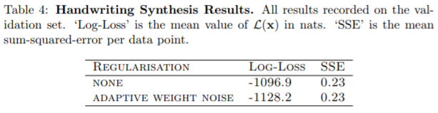
Table 4 shows that adaptive weight noise gave a considerable improvement in log-loss (around 31.3 nats) but no significant change in sum-squared error. The regularised network appears to generate slightly more realistic sequences, although the difference is hard to discern by eye. Both networks performed considerably better than the best prediction network. In particular the sumsquared-error was reduced by 44%. This is likely due in large part to the improved predictions at the ends of strokes, where the error is largest	表4显示，自适应权值噪声在对数损失(约31.3 nats)方面有显著改善，但在平方和误差方面没有显著变化。这个规则化的网络似乎产生了更真实的序列，尽管这种差异很难用肉眼辨别。这两个网络都比最佳预测网络表现得好得多。特别是sumsquared-error减少了44%。这可能在很大程度上是由于改进了笔画末端的预测，在那里误差最大

5.3 Unbiased Sampling 公正的抽样

Given c, an unbiased sample can be picked from Pr(x|c) by iteratively drawing xt+1 from Pr (xt+1|yt), just as for the prediction network. The only difference is that we must also decide when the synthesis network has finished writing the text and should stop making any future decisions. To do this, we use the following heuristic: as soon as φ(t, U + 1) > φ(t, u) ∀ 1 ≤ u ≤ U the current input xt is defined as the end of the sequence and sampling ends. Examples of unbiased synthesis samples are shown in Fig. 15. These and all subsequent figures were generated using the synthesis network retrained with adaptive weight noise. Notice how stylistic traits, such as character size, slant, cursiveness etc. vary widely between the samples, but remain more-or-less consistent within them. This suggests that the network identifies the traits early on in the sequence, then remembers them until the end. By looking through enough samples for a given text, it appears to be possible to find virtually any combination of stylistic traits, which suggests that the network models them independently both from each other and from the text. ‘

给定c，从Pr(x|c)中迭代提取xt+1从Pr(xt+1|yt)中提取无偏样本，与预测网络一样。唯一不同的是，我们还必须决定合成网络何时完成文本的编写，并且应该停止做任何未来的决定。为此,我们使用以下启发式:一旦φ(t, U + 1) >φ(t, U)∀1≤≤U当前输入xt被定义为序列图和采样结束的结束。无偏合成样本的例子如图15所示。这些和所有后续的图像都是使用自适应权值噪声再训练的合成网络生成的。请注意，风格特征，如字符大小、倾斜度、曲线性等，在不同的样本之间差异很大，但在样本内部却或多或少保持一致。这表明，该网络在序列的早期识别出这些特征，然后记住它们，直到最后。通过对给定文本的足够多的样本进行研究，似乎有可能发现几乎任何风格特征的组合，这表明网络对它们进行独立建模，既相互独立，也独立于文本。”

Blind taste tests’ carried out by the author during presentations suggest that at least some unbiased samples cannot be distinguished from real handwriting by the human eye. Nonetheless the network does make mistakes we would not expect a human writer to make, often involving missing, confused or garbled letters3 ; this suggests that the network sometimes has trouble determining the alignment between the characters and the trace. The number of mistakes increases markedly when less common words or phrases are included in the character sequence. Presumably this is because the network learns an implicit character-level language model from the training set that gets confused when rare or unknown transitions occur.

作者在演讲中进行的盲品测试表明，至少有一些没有偏见的样品无法通过肉眼分辨出真迹。尽管如此，网络确实会犯一些我们不希望人类作家会犯的错误，通常包括丢失、混淆或含混的信件;这表明，网络有时难以确定字符和跟踪之间的对齐。当较不常见的单词或短语被包含在字符序列中时，错误数量显著增加。这可能是因为当罕见或未知的转换发生时，网络会从训练集中学习隐式的字符级语言模型。

5.4 Biased Sampling 有偏见的抽样

One problem with unbiased samples is that they tend to be difficult to read (partly because real handwriting is difficult to read, and partly because the network is an imperfect model). Intuitively, we would expect the network to give higher probability to good handwriting because it tends to be smoother and more predictable than bad handwriting. If this is true, we should aim to output more probable elements of Pr(x|c) if we want the samples to be easier to read. A principled search for high probability samples could lead to a difficult inference problem, as the probability of every output depends on all previous outputs. However a simple heuristic, where the sampler is biased towards more probable predictions at each step independently, generally gives good results. Define the probability bias b as a real number greater than or equal to zero. Before drawing a sample from Pr(xt+1|yt), each standard deviation σ j t in the Gaussian mixture is recalculated from Eq. (21) to

无偏样本的一个问题是它们往往难以阅读(部分原因是真实的笔迹难以阅读，部分原因是网络模型不完善)。直觉上，我们认为网络会给好笔迹更高的概率，因为它比糟糕的笔迹更平滑、更可预测。如果这是真的，我们应该输出更多可能的元素Pr(x|c)，如果我们想让样本更容易阅读。对高概率样本的原则性搜索可能会导致一个困难的推理问题，因为每个输出的概率依赖于所有以前的输出。然而，一个简单的启发式，其中采样器是偏向于更可能的预测，在每一步独立，通常会给出良好的结果。将概率偏差b定义为大于或等于零的实数。之前图纸样本公关(xt + 1 |次),每一个标准差σj t在高斯混合重新计算从情商。(21)

This artificially reduces the variance in both the choice of component from the mixture, and in the distribution of the component itself. When b = 0 unbiased sampling is recovered, and as b → ∞ the variance in the sampling disappears and the network always outputs the mode of the most probable component in the mixture (which is not necessarily the mode of the mixture, but at least a reasonable approximation). Fig. 16 shows the effect of progressively increasing the bias, and Fig. 17 shows samples generated with a low bias for the same texts as Fig. 15.

这就人为地减少了混合中组分的选择和组分本身分布的差异。b = 0时的采样恢复,当b→∞方差在抽样消失,网络总是输出模式最可能的组件的混合物(不一定是混合的模式,但至少有一个合理的近似)。图16为逐步增大偏倚的效果，图17为与图15相同文本产生的低偏倚样本。

5.5 Primed Sampling 启动采样

Another reason to constrain the sampling would be to generate handwriting in the style of a particular writer (rather than in a randomly selected style). The easiest way to do this would be to retrain it on that writer only. But even without retraining, it is possible to mimic a particular style by ‘priming’ the network with a real sequence, then generating an extension with the real sequence still in the network’s memory. This can be achieved for a real x, c and a synthesis character string s by setting the character sequence to c 0 = c + s and clamping the data inputs to x for the first T timesteps, then sampling as usual until the sequence ends. Examples of primed samples are shown in Figs. 18 and 19. The fact that priming works proves that the network is able to remember stylistic features identified earlier on in the sequence. This technique appears to work better for sequences in the training data than those the network has never seen.	限制抽样的另一个原因是生成特定作者风格的笔迹(而不是随机选择的风格)。最简单的方法是只对那个编写器进行再培训。但是，即使不进行再训练，也可以通过用真实序列“启动”网络来模仿特定的样式，然后生成一个扩展，其中真实序列仍然保留在网络的内存中。这可以通过将字符序列设置为c 0 = c + s，并在第一个T时间步将数据输入固定到x，然后像往常一样采样，直到序列结束，从而实现对实际的x、c和合成字符串s的采样。启动样本的例子如图18和图19所示。启动起作用的事实证明，网络能够记住在序列前面识别出的文体特征。这种技术似乎比网络从未见过的序列更适合训练数据。
Primed sampling and reduced variance sampling can also be combined. As shown in Figs. 20 and 21 this tends to produce samples in a ‘cleaned up’ version of the priming style, with overall stylistic traits such as slant and cursiveness retained, but the strokes appearing smoother and more regular. A possible application would be the artificial enhancement of poor handwriting.	启动抽样和减少方差抽样也可以结合使用。如图20和图21所示，这往往会产生一种“净化”版的引语风格，保留了整体风格特征，如倾斜度和曲线感，但笔触看起来更平滑、更有规则。一种可能的应用是人为地改进拙劣的笔迹。

6 Conclusions and Future Work 结论与未来工作

This paper has demonstrated the ability of Long Short-Term Memory recurrent neural networks to generate both discrete and real-valued sequences with complex, long-range structure using next-step prediction. It has also introduced a novel convolutional mechanism that allows a recurrent network to condition its predictions on an auxiliary annotation sequence, and used this approach to synthesise diverse and realistic samples of online handwriting. Furthermore, it has shown how these samples can be biased towards greater legibility, and how they can be modelled on the style of a particular writer.

本文证明了长短时记忆递归神经网络利用下一步预测生成具有复杂、长时程结构的离散和实值序列的能力。它还引入了一种新颖的卷积机制，允许递归网络根据辅助注释序列调整预测，并使用这种方法来合成各种真实的在线手写样本。此外，它还展示了这些样本如何倾向于更大的易读性，以及如何模仿特定作者的风格。

Several directions for future work suggest themselves. One is the application of the network to speech synthesis, which is likely to be more challenging than handwriting synthesis due to the greater dimensionality of the data points. Another is to gain a better insight into the internal representation of the data, and to use this to manipulate the sample distribution directly. It would also be interesting to develop a mechanism to automatically extract high-level annotations from sequence data. In the case of handwriting, this could allow for more nuanced annotations than just text, for example stylistic features, different forms of the same letter, information about stroke order and so on.

未来的工作有几个方向。一是网络在语音合成中的应用，由于数据点的维数较大，语音合成可能比手写合成更具挑战性。另一种方法是更好地了解数据的内部表示形式，并使用它直接操纵样本分布。开发一种从序列数据中自动提取高级注释的机制也很有趣。在书写的情况下，这可能允许比文本更微妙的注释，例如风格特征，同一字母的不同形式，关于笔画顺序的信息等等。

Acknowledgements 致谢

Thanks to Yichuan Tang, Ilya Sutskever, Navdeep Jaitly, Geoffrey Hinton and other colleagues at the University of Toronto for numerous useful comments and suggestions. This work was supported by a Global Scholarship from the Canadian Institute for Advanced Research.

感谢多伦多大学的Yichuan Tang, Ilya Sutskever, Navdeep Jaitly, Geoffrey Hinton和其他同事提供了许多有用的意见和建议。这项工作得到了加拿大高级研究所的全球奖学金的支持。

References

[1] Y. Bengio, P. Simard, and P. Frasconi. Learning long-term dependencies with gradient descent is difficult. IEEE Transactions on Neural Networks, 5(2):157–166, March 1994.
[2] C. Bishop. Mixture density networks. Technical report, 1994.
[3] C. Bishop. Neural Networks for Pattern Recognition. Oxford University Press, Inc., 1995.
[4] N. Boulanger-Lewandowski, Y. Bengio, and P. Vincent. Modeling temporal dependencies in high-dimensional sequences: Application to polyphonic music generation and transcription. In Proceedings of the Twenty-nine International Conference on Machine Learning (ICML’12), 2012.
[5] J. G. Cleary, Ian, and I. H. Witten. Data compression using adaptive coding and partial string matching. IEEE Transactions on Communications, 32:396–402, 1984.
[6] D. Eck and J. Schmidhuber. A first look at music composition using lstm recurrent neural networks. Technical report, IDSIA USI-SUPSI Instituto Dalle Molle.
[7] F. Gers, N. Schraudolph, and J. Schmidhuber. Learning precise timing with LSTM recurrent networks. Journal of Machine Learning Research, 3:115–143, 2002.
[8] A. Graves. Practical variational inference for neural networks. In Advances in Neural Information Processing Systems, volume 24, pages 2348–2356. 2011.
[9] A. Graves. Sequence transduction with recurrent neural networks. In ICML Representation Learning Worksop, 2012.
[10] A. Graves, A. Mohamed, and G. Hinton. Speech recognition with deep recurrent neural networks. In Proc. ICASSP, 2013.
[11] A. Graves and J. Schmidhuber. Framewise phoneme classification with bidirectional LSTM and other neural network architectures. Neural Networks, 18:602–610, 2005.
[12] A. Graves and J. Schmidhuber. Offline handwriting recognition with multidimensional recurrent neural networks. In Advances in Neural Information Processing Systems, volume 21, 2008.
[13] P. D. Gr¨unwald. The Minimum Description Length Principle (Adaptive Computation and Machine Learning). The MIT Press, 2007.
[14] G. Hinton. A Practical Guide to Training Restricted Boltzmann Machines. Technical report, 2010.
[15] S. Hochreiter, Y. Bengio, P. Frasconi, and J. Schmidhuber. Gradient Flow in Recurrent Nets: the Difficulty of Learning Long-term Dependencies. In S. C. Kremer and J. F. Kolen, editors, A Field Guide to Dynamical Recurrent Neural Networks. 2001.
[16] S. Hochreiter and J. Schmidhuber. Long Short-Term Memory. Neural Computation, 9(8):1735–1780, 1997.
[17] M. Hutter. The Human Knowledge Compression Contest, 2012. [18] K.-C. Jim, C. Giles, and B. Horne. An analysis of noise in recurrent neural networks: convergence and generalization. Neural Networks, IEEE Transactions on, 7(6):1424 –1438, 1996. [19] S. Johansson, R. Atwell, R. Garside, and G. Leech. The tagged LOB corpus user’s manual; Norwegian Computing Centre for the Humanities, 1986.
[20] B. Knoll and N. de Freitas. A machine learning perspective on predictive coding with paq. CoRR, abs/1108.3298, 2011.
[21] M. Liwicki and H. Bunke. IAM-OnDB - an on-line English sentence database acquired from handwritten text on a whiteboard. In Proc. 8th Int. Conf. on Document Analysis and Recognition, volume 2, pages 956– 961, 2005.
[22] M. P. Marcus, B. Santorini, and M. A. Marcinkiewicz. Building a large annotated corpus of english: The penn treebank. COMPUTATIONAL LINGUISTICS, 19(2):313–330, 1993.
[23] T. Mikolov. Statistical Language Models based on Neural Networks. PhD thesis, Brno University of Technology, 2012.
[24] T. Mikolov, I. Sutskever, A. Deoras, H. Le, S. Kombrink, and J. Cernocky. Subword language modeling with neural networks. Technical report, Unpublished Manuscript, 2012.
[25] A. Mnih and G. Hinton. A Scalable Hierarchical Distributed Language Model. In Advances in Neural Information Processing Systems, volume 21, 2008.
[26] A. Mnih and Y. W. Teh. A fast and simple algorithm for training neural probabilistic language models. In Proceedings of the 29th International Conference on Machine Learning, pages 1751–1758, 2012.
[27] T. N. Sainath, A. Mohamed, B. Kingsbury, and B. Ramabhadran. Lowrank matrix factorization for deep neural network training with highdimensional output targets. In Proc. ICASSP, 2013.
[28] M. Schuster. Better generative models for sequential data problems: Bidirectional recurrent mixture density networks. pages 589–595. The MIT Press, 1999.
[29] I. Sutskever, G. E. Hinton, and G. W. Taylor. The recurrent temporal restricted boltzmann machine. pages 1601–1608, 2008.
[30] I. Sutskever, J. Martens, and G. Hinton. Generating text with recurrent neural networks. In ICML, 2011.
[31] G. W. Taylor and G. E. Hinton. Factored conditional restricted boltzmann machines for modeling motion style. In Proc. 26th Annual International Conference on Machine Learning, pages 1025–1032, 2009.
[32] T. Tieleman and G. Hinton. Lecture 6.5 - rmsprop: Divide the gradient by a running average of its recent magnitude, 2012.
[33] R. Williams and D. Zipser. Gradient-based learning algorithms for recurrent networks and their computational complexity. In Back-propagation: Theory, Architectures and Applications, pages 433–486. 1995.

点赞 2
收藏
分享
文章举报

一个处女座的程序猿博客专家发布了1623 篇原创文章 · 获赞 6721 · 访问量 1295万+ 他的留言板关注

内容来自用户分享和网络整理，不保证内容的准确性，如有侵权内容，可联系管理员处理

标签：

相关文章推荐

新的分享

章节导航