任务2·逻辑回归算法整理

逻辑回归与线性回归

联系

逻辑回归与线性回归都属于广义线性回归模型。

逻辑回归往往是解决二元0/1分类问题的，之所以叫“回归”因为其本质还是线性回归。可以认为逻辑回归的输入是线性回归的输出，将逻辑斯蒂函数（Sigmoid曲线）作用于线性回归的输出得到输出结果。

• 线性回归y = ax + b, 其中a和b是待求参数；
• 逻辑回归p = S(ax + b), 其中a和b是待求参数， S是逻辑斯蒂函数，然后根据p与1-p的大小确定输出的值，通常阈值取0.5，若p大于0.5则归为1这类。

区别

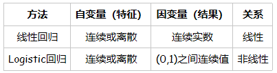
1. 线性回归目标函数是最小二乘，而逻辑回归则是似然函数。也正是因为使用的参数估计的方法不同，线性回归模型更容易受到异常值(outlier)的影响，有可能需要不断变换阈值(threshold)；
2. 线性回归是在整个实数域范围内进行预测，敏感度一致。逻辑回归则将预测值限定为[0,1]间。因而对于这类问题来说，逻辑回归的鲁棒性比线性回归的要好。
   
3. 线性回归中，独立变量的系数解释十分明了，就是保持其他变量不变时，改变单个变量因变量的改变量。逻辑回归中，自变量系数的解释就要视情况而定了，要看选用的概率分布是什么，如二项式分布，泊松分布等。

逻辑回归的原理

以二元逻辑回归为例

逻辑回归损失函数推导及优化

逻辑回归采用交叉熵作为代价函数，即对数损失函数（logarithmic loss function) 或对数似然损失函数(log-likehood loss function)：

L(Y,P(Y|X))=−logP(Y|X)

对数损失函数能够有效避免梯度消失。

对于二元逻辑回归的损失函数极小化，有比较多的方法，最常见的有梯度下降法，坐标轴下降法，等牛顿法等。这里推导出梯度下降法中θ每次迭代的公式。由于代数法推导比较的繁琐，我习惯于用矩阵法来做损失函数的优化过程，这里给出矩阵法推导二元逻辑回归梯度的过程。

正则化与模型评估指标

逻辑回归的L1正则化的损失函数表达式如下，相比普通的逻辑回归损失函数，增加了L1的范数做作为惩罚，超参数α作为惩罚系数，调节惩罚项的大小。

模型评估指标：

• 精准率
• 召回率
• F1 score
• precision—recall的平衡（曲线）
• ROC曲线

详情参考：逻辑回归及其评价指标——自学第九篇
https://blog.csdn.net/yh_1021/article/details/82765923

逻辑回归的优缺点

优点：

1、实现简单；

2、分类时计算量非常小，速度很快，存储资源低；

缺点：

1、容易欠拟合，一般准确度不太高；

2、只能处理两分类问题（在此基础上衍生出来的softmax可以用于多分类），且必须线性可分；

样本不均衡问题解决办法

处理样本不均衡数据一般可以有以下方法：

1、人为将样本变为均衡数据。

上采样：重复采样样本量少的部分，以数据量多的一方的样本数量为标准，把样本数量较少的类的样本数量生成和样本数量多的一方相同。

下采样：减少采样样本量多的部分，以数据量少的一方的样本数量为标准。

2、调节模型参数（class_weigh，sample_weight，这些参数不是对样本进行上采样下采样等处理，而是在损失函数上对不同的样本加上权重）

（A）逻辑回归中的参数class_weigh；

在逻辑回归中，参数class_weight默认None，此模式表示假设数据集中的所有标签是均衡的，即自动认为标签的比例是1：1。所以当样本不均衡的时候，我们可以使用形如{标签的值1：权重1，标签的值2：权重2}的字典来输入真实的样本标签比例（例如{“违约”：10，“未违约”：1}），来提高违约样本在损失函数中的权重。

或者使用”balanced“模式，sklearn内部原理：直接使用n_samples/(n_classes * np.bincount(y))，即样本总数/(类别数量*y0出现频率)作为权重，可以比较好地修正我们的样本不均衡情况。

sklearn参数

代码实现：

#Import Library
#Import other necessary libraries like pandas, numpy...
from sklearn import linear_model
#Load Train and Test datasets
#Identify feature and response variable(s) and values must be numeric and numpy arrays

x_train=input_variables_values_training_datasets
y_train=target_variables_values_training_datasets
x_test=input_variables_values_test_datasets

# Create linear regression object
linear = linear_model.LinearRegression()

# Train the model using the training sets and check score
linear.fit(x_train, y_train)
linear.score(x_train, y_train)

#Equation coefficient and Intercept
print('Coefficient: \n', linear.coef_)
print('Intercept: \n', linear.intercept_)

#Predict Output
predicted= linear.predict(x_test)

上述是使用sklearn包中的线性回归算法的代码例子，下面是一个实现的具体例子。

# -*- coding: utf-8 -*-
"""
Created on Mon Oct 17 10:36:06 2016

@author: cai
"""

import os
import numpy as np
import pandas as pd
import matplotlib.pylab as plt
from sklearn import linear_model

# 计算损失函数
def computeCost(X, y, theta):
inner = np.power(((X * theta.T) - y), 2)
return np.sum(inner) / (2 * len(X))

# 梯度下降算法
def gradientDescent(X, y, theta, alpha, iters):
temp = np.matrix(np.zeros(theta.shape))
parameters = int(theta.ravel().shape[1])
cost = np.zeros(iters)

for i in range(iters):
error = (X * theta.T) - y

for j in range(parameters):
# 计算误差对权值的偏导数
term = np.multiply(error, X[:, j])
# 更新权值
temp[0, j] = theta[0, j] - ((alpha / len(X)) * np.sum(term))

theta = temp
cost[i] = computeCost(X, y, theta)
return theta, cost

dataPath = os.path.join('data', 'ex1data1.txt')
data = pd.read_csv(dataPath, header=None, names=['Population', 'Profit'])
# print(data.head())
# print(data.describe())
# data.plot(kind='scatter', x='Population', y='Profit', figsize=(12, 8))
# 在数据起始位置添加1列数值为1的数据
data.insert(0, 'Ones', 1)
print(data.shape)

cols = data.shape[1]
X = data.iloc[:, 0:cols-1]
y = data.iloc[:, cols-1:cols]

# 从数据帧转换成numpy的矩阵格式
X = np.matrix(X.values)
y = np.matrix(y.values)
# theta = np.matrix(np.array([0, 0]))
theta = np.matrix(np.zeros((1, cols-1)))
print(theta)
print(X.shape, theta.shape, y.shape)
cost = computeCost(X, y, theta)
print("cost = ", cost)

# 初始化学习率和迭代次数
alpha = 0.01
iters = 1000

# 执行梯度下降算法
g, cost = gradientDescent(X, y, theta, alpha, iters)
print(g)

# 可视化结果
x = np.linspace(data.Population.min(),data.Population.max(),100)
f = g[0, 0] + (g[0, 1] * x)

fig, ax = plt.subplots(figsize=(12, 8))
ax.plot(x, f, 'r', label='Prediction')
ax.scatter(data.Population, data.Profit, label='Training Data')
ax.legend(loc=2)
ax.set_xlabel('Population')
ax.set_ylabel('Profit')
ax.set_title('Predicted Profit vs. Population Size')

fig, ax = plt.subplots(figsize=(12, 8))
ax.plot(np.arange(iters), cost, 'r')
ax.set_xlabel('Iteration')
ax.set_ylabel('Cost')
ax.set_title('Error vs. Training Epoch')

# 使用sklearn 包里面实现的线性回归算法
model = linear_model.LinearRegression()
model.fit(X, y)

x = np.array(X[:, 1].A1)
# 预测结果
f = model.predict(X).flatten()
# 可视化
fig, ax = plt.subplots(figsize=(12, 8))
ax.plot(x, f, 'r', label='Prediction')
ax.scatter(data.Population, data.Profit, label='Training Data')
ax.legend(loc=2)
ax.set_xlabel('Population')
ax.set_ylabel('Profit')
ax.set_title('Predicted Profit vs. Population Size(using sklearn)')
plt.show()

参考：
刘建平Pinard https://www.geek-share.com/detail/2689265720.html
逻辑回归与线性回归的区别与联系 https://blog.csdn.net/lx_ros/article/details/81263209
处理样本不均衡数据 https://www.cnblogs.com/simpleDi/p/10235907.html
机器学习sklearn19.0——Logistic回归算法 https://www.geek-share.com/detail/2724476610.html
机器学习算法总结–线性回归和逻辑回归 https://www.geek-share.com/detail/2697897372.html