matlab简单图像预处理

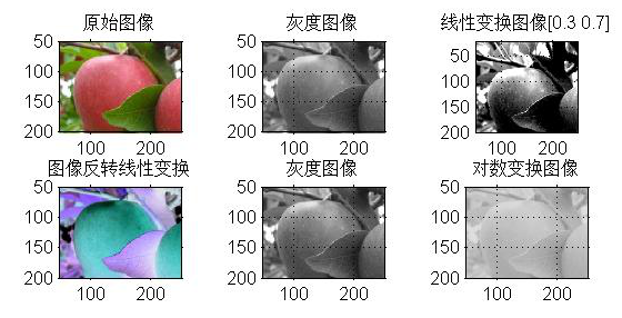
转自https://blog.csdn.net/renyp8799/article/details/51191692，很实用的简单操作，适合图像处理初学者一、图像反转[plain] view plain copyI=imread('input_image.jpg');  
J=double(I);  
J=-J+(256-1); %图像反转线性变换  
H=uint8(J);  
subplot(3,3,4),imshow(H);  
title('图像反转线性变换');  
axis([50,250,50,200]);  
axis on;  

二、灰度线性变换[plain] view plain copyI=imread('input_image.jpg');  
subplot(3,3,1),imshow(I);  
title('原始图像');  
axis([50,250,50,200]);  
axis on;  
  
I1 = rgb2gray(I);  
subplot(3,3,2),imshow(I1)  
title('灰度图像')  
axis([50,250,50,200]);  
grid on;  
axis on;  
K=imadjust(I1,[0.3 0.7],[]);  
subplot(3,3,3),imshow(K);  
title('线性变换图像[0.3 0.7]');  
axis([50,250,20,200]);  
grid on;  
axis on;  
三、非线性变换[plain] view plain copyI=imread('input_image.jpg');  
I1 = rgb2gray(I);  
subplot(3,3,5),imshow(I1);  
title('灰度图像');  
axis([50,250,50,200]);  
grid on; %显示网格线  
axis on; %显示坐标系  
J=double(I1);  
J=40*(log(J+1));  
H=uint8(J);  
subplot(3,3,6),imshow(H);  
title('对数变换图像');  
axis([50,250,50,200]);  
grid on; %显示网格线  
axis on; %显示坐标系  
上述代码结果：


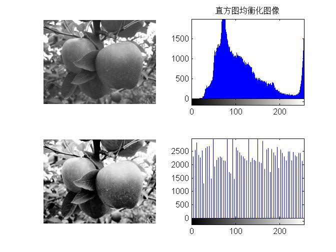
四、直方图均衡化[plain] view plain copyI=imread('input_image.jpg');  
figure;  
I=rgb2gray(I);  
subplot(2,2,1);  
imshow(I);  
   
subplot(2,2,2);  
imhist(I);  
title('直方图均衡化图像');  
   
I1 = histeq(I);  
subplot(2,2,3);  
imshow(I1);  
subplot(2,2,4);  
imhist(I1);  
上述代码结果：


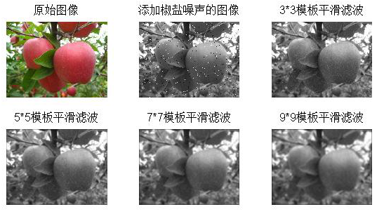
五、线性平滑滤波器
[plain] view plain copyI=imread('input_image.jpg');  
figure;  
subplot(231)  
imshow(I)  
title('原始图像')  
I=rgb2gray(I);  
I1=imnoise(I,'salt & pepper',0.02);  
subplot(232)  
imshow(I1)  
title('添加椒盐噪声的图像')  
   
k1=filter2(fspecial('average',3),I1)/255; %进行3*3模板平滑滤波  
k2=filter2(fspecial('average',5),I1)/255; %进行5*5模板平滑滤波  
k3=filter2(fspecial('average',7),I1)/255; %进行7*7模板平滑滤波  
k4=filter2(fspecial('average',9),I1)/255; %进行9*9模板平滑滤波  
subplot(233),imshow(k1);title('3*3模板平滑滤波');  
subplot(234),imshow(k2);title('5*5模板平滑滤波');  
subplot(235),imshow(k3);title('7*7模板平滑滤波');  
subplot(236),imshow(k4);title('9*9模板平滑滤波');  
上述代码结果：



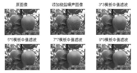
六、中值滤波器[plain] view plain copyfigure;  
I=imread('input_image.jpg');  
I=rgb2gray(I);  
subplot(231),imshow(I);  
title('原图像');  
   
J=imnoise(I,'salt & pepper',0.02);  
subplot(232),imshow(J);  
title('添加椒盐噪声图像');  
   
k1=medfilt2(J); %进行3*3模板中值滤波  
k2=medfilt2(J,[5,5]); %进行5*5模板中值滤波  
k3=medfilt2(J,[7,7]); %进行7*7模板中值滤波  
k4=medfilt2(J,[9,9]); %进行9*9模板中值滤波  
subplot(233),imshow(k1);title('3*3模板中值滤波');  
subplot(234),imshow(k2);title('5*5模板中值滤波');  
subplot(235),imshow(k3);title('7*7模板中值滤波');  
subplot(236),imshow(k4);title('9*9模板中值滤波');  
上述代码结果：



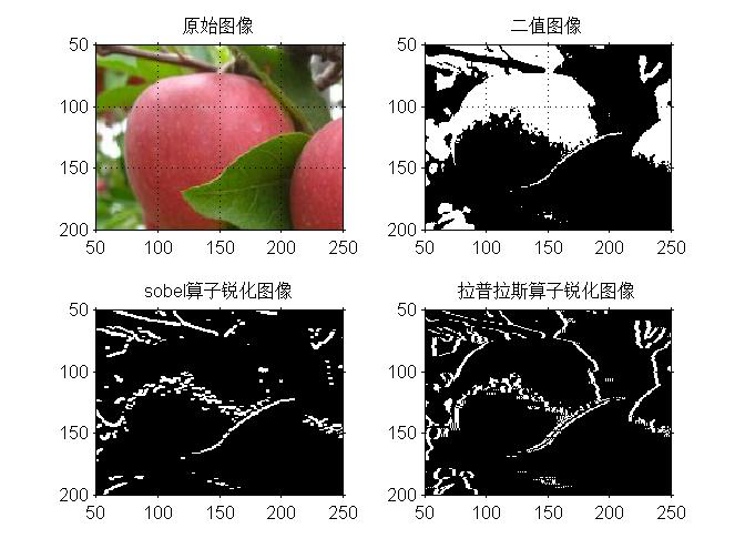
七、用Sobel算子和拉普拉斯对图像锐化[plain] view plain copyfigure;  
I=imread('input_image.jpg');  
subplot(2,2,1),imshow(I);  
title('原始图像');  
axis([50,250,50,200]);  
grid on; %显示网格线  
axis on; %显示坐标系  
I1=im2bw(I);  
subplot(2,2,2),imshow(I1);  
title('二值图像');  
axis([50,250,50,200]);  
grid on; %显示网格线  
axis on; %显示坐标系  
H=fspecial('sobel'); %选择sobel算子  
J=filter2(H,I1); %卷积运算  
subplot(2,2,3),imshow(J);  
title('sobel算子锐化图像');  
axis([50,250,50,200]);  
grid on; %显示网格线  
axis on; %显示坐标系  
   
I1 = double(I1);  
h=[0 1 0,1 -4 1,0 1 0]; %拉普拉斯算子  
J1=conv2(I1,h,'same'); %卷积运算  
subplot(2,2,4),imshow(J1);  
title('拉普拉斯算子锐化图像');  
axis([50,250,50,200]);  
grid on; %显示网格线  
axis on; %显示坐标系  
上述代码结果：



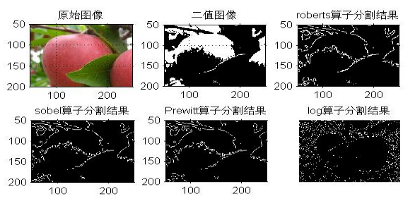
八、梯度算子检测边缘[plain] view plain copyfigure;  
I=imread('input_image.jpg');  
subplot(2,3,1);  
imshow(I);  
title('原始图像');  
axis([50,250,50,200]);  
grid on; %显示网格线  
axis on; %显示坐标系  
I1=im2bw(I);  
subplot(2,3,2);  
imshow(I1);  
title('二值图像');  
axis([50,250,50,200]);  
grid on; %显示网格线  
axis on; %显示坐标系  
I2=edge(I1,'roberts');  
   
subplot(2,3,3);  
imshow(I2);  
title('roberts算子分割结果');  
axis([50,250,50,200]);  
grid on; %显示网格线  
axis on; %显示坐标系  
I3=edge(I1,'sobel');  
subplot(2,3,4);  
imshow(I3);  
title('sobel算子分割结果');  
axis([50,250,50,200]);  
grid on; %显示网格线  
axis on; %显示坐标系  
I4=edge(I1,'Prewitt');  
subplot(2,3,5);  
imshow(I4);  
title('Prewitt算子分割结果');  
axis([50,250,50,200]);  
grid on; %显示网格线  
axis on; %显示坐标系  
九、LOG算子检测边缘
[plain] view plain copyI1=rgb2gray(I);  
I2=edge(I1,'log');  
subplot(2,3,6);  
imshow(I2);  
title('log算子分割结果');  
上述代码结果：



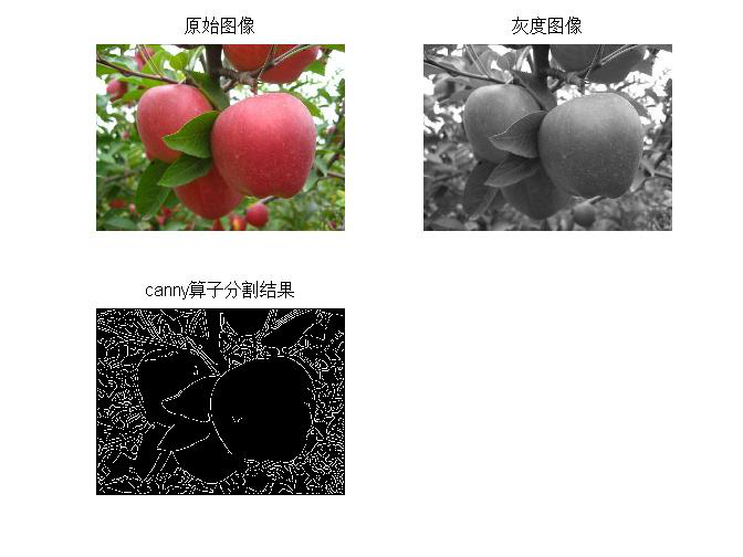
十、Canny算子检测边缘
[plain] view plain copyfigure;  
I=imread('input_image.jpg');  
subplot(2,2,1);  
imshow(I);  
title('原始图像')  
I1=rgb2gray(I);  
subplot(2,2,2);  
imshow(I1);  
title('灰度图像');  
I2=edge(I1,'canny');  
subplot(2,2,3);  
imshow(I2);  
title('canny算子分割结果');  
上述代码结果：


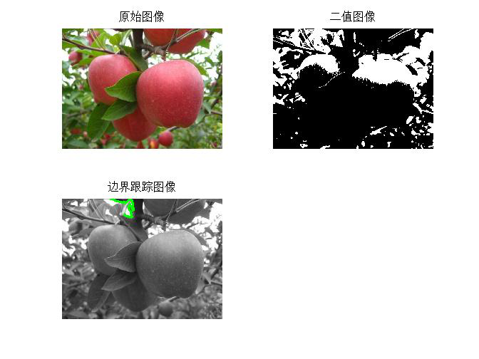
十一、边界跟踪（bwtraceboundary函数）

[plain] view plain copyI=imread('input_image.jpg');  
figure  
subplot(2,2,1);  
imshow(I);  
title('原始图像');  
   
I1=rgb2gray(I); %将彩色图像转化灰度图像  
threshold=graythresh(I1); %计算将灰度图像转化为二值图像所需的门限  
BW=im2bw(I1, threshold); %将灰度图像转化为二值图像  
subplot(2,2,2);  
imshow(BW);  
title('二值图像');  
   
dim=size(BW);  
col=round(dim(2)/2)-90; %计算起始点列坐标  
row=find(BW(:,col),1); %计算起始点行坐标  
connectivity=8;  
num_points=180;  
contour=bwtraceboundary(BW,[row,col],'N',connectivity,num_points);  
%提取边界  
subplot(2,2,3);  
imshow(I1);  
hold on;  
plot(contour(:,2),contour(:,1), 'g','LineWidth' ,2);  
title('边界跟踪图像');  
上述代码结果：



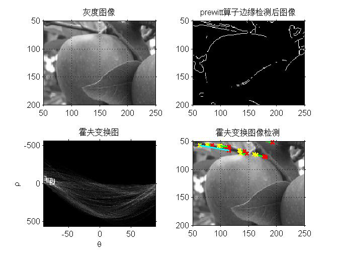
十二、Hough变换

[plain] view plain copyfigure;  
I=imread('input_image.jpg');  
rotI=rgb2gray(I);  
subplot(2,2,1);  
imshow(rotI);  
title('灰度图像');  
axis([50,250,50,200]);  
grid on;  
axis on;  
BW=edge(rotI,'prewitt');  
subplot(2,2,2);  
imshow(BW);  
title('prewitt算子边缘检测后图像');  
axis([50,250,50,200]);  
grid on;  
axis on;  
[H,T,R]=hough(BW);  
subplot(2,2,3);  
imshow(H,[],'XData',T,'YData',R,'InitialMagnification','fit');  
title('霍夫变换图');  
xlabel('\theta'),ylabel('\rho');  
axis on , axis normal, hold on;  
P=houghpeaks(H,5,'threshold',ceil(0.3*max(H(:))));  
x=T(P(:,2));y=R(P(:,1));  
plot(x,y,'s','color','white');  
lines=houghlines(BW,T,R,P,'FillGap',5,'MinLength',7);  
subplot(2,2,4);imshow(rotI);  
title('霍夫变换图像检测');  
axis([50,250,50,200]);  
grid on;  
axis on;  
hold on;  
max_len=0;  
for k=1:length(lines)  
xy=[lines(k).point1;lines(k).point2];  
plot(xy(:,1),xy(:,2),'LineWidth',2,'Color','green');  
plot(xy(1,1),xy(1,2),'x','LineWidth',2,'Color','yellow');  
plot(xy(2,1),xy(2,2),'x','LineWidth',2,'Color','red');  
len=norm(lines(k).point1-lines(k).point2);  
if(len>max_len)  
max_len=len;  
xy_long=xy;  
end  
end  
plot(xy_long(:,1),xy_long(:,2),'LineWidth',2,'Color','cyan');  
上述代码结果：



十三、直方图阈值法[plain] view plain copyfigure;  
I=imread('input_image.jpg');  
I1=rgb2gray(I);  
subplot(2,2,1);  
imshow(I1);  
title('灰度图像')  
axis([50,250,50,200]);  
grid on; %显示网格线  
axis on; %显示坐标系  
[m,n]=size(I1); %测量图像尺寸参数  
GP=zeros(1,256); %预创建存放灰度出现概率的向量  
for k=0:255  
GP(k+1)=length(find(I1==k))/(m*n); %计算每级灰度出现的概率，将其存入GP中相应位置  
end  
subplot(2,2,2),bar(0:255,GP,'g') %绘制直方图  
title('灰度直方图')  
xlabel('灰度值')  
ylabel('出现概率')  
I2=im2bw(I,150/255);  
subplot(2,2,3),imshow(I2);  
title('阈值150的分割图像')  
axis([50,250,50,200]);  
grid on; %显示网格线  
axis on; %显示坐标系  
I3=im2bw(I,200/255); %  
subplot(2,2,4),imshow(I3);  
title('阈值200的分割图像')  
axis([50,250,50,200]);  
grid on; %显示网格线  
axis on; %显示坐标系  
上述代码结果：



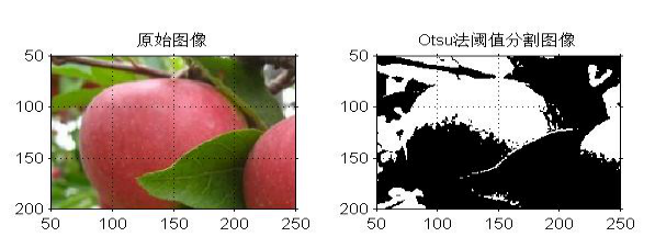
十四、自动阈值法：Otsu法[plain] view plain copyclc  
clear all  
figure;  
I=imread('input_image.jpg');  
subplot(1,2,1),imshow(I);  
title('原始图像')  
axis([50,250,50,200]);  
grid on; %显示网格线  
axis on; %显示坐标系  
level=graythresh(I); %确定灰度阈值  
BW=im2bw(I,level);  
subplot(1,2,2),imshow(BW);  
title('Otsu法阈值分割图像')  
axis([50,250,50,200]);  
grid on; %显示网格线  
axis on; %显示坐标系  
上述代码结果：



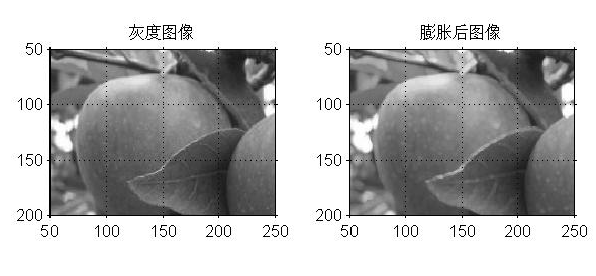
十五、膨胀操作[plain] view plain copyfigure;  
I=imread('input_image.jpg');  
I1=rgb2gray(I);  
subplot(1,2,1);  
imshow(I1);  
title('灰度图像')  
axis([50,250,50,200]);  
grid on; %显示网格线  
axis on; %显示坐标系  
se=strel('disk',1); %生成圆形结构元素  
I2=imdilate(I1,se); %用生成的结构元素对图像进行膨胀  
subplot(1,2,2);  
imshow(I2);  
title('膨胀后图像');  
axis([50,250,50,200]);  
grid on; %显示网格线  
axis on; %显示坐标系  
上述代码结果：



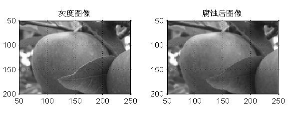
十六、腐蚀操作[plain] view plain copyfigure;  
I=imread('input_image.jpg');  
I1=rgb2gray(I);  
subplot(1,2,1);  
imshow(I1);  
title('灰度图像')  
axis([50,250,50,200]);  
grid on; %显示网格线  
axis on; %显示坐标系  
se=strel('disk',1); %生成圆形结构元素  
I2=imerode(I1,se); %用生成的结构元素对图像进行腐蚀  
subplot(1,2,2);  
imshow(I2);  
title('腐蚀后图像');  
axis([50,250,50,200]);  
grid on; %显示网格线  
axis on; %显示坐标系  
上述代码结果：



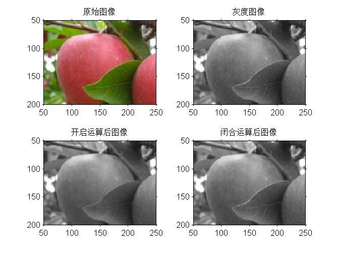
十七、开启和闭合操作[plain] view plain copyfigure;  
I=imread('input_image.jpg');  
subplot(2,2,1),imshow(I);  
title('原始图像');  
axis([50,250,50,200]);  
axis on; %显示坐标系  
I1=rgb2gray(I);  
subplot(2,2,2),imshow(I1);  
title('灰度图像');  
axis([50,250,50,200]);  
axis on; %显示坐标系  
se=strel('disk',1); %采用半径为1的圆作为结构元素  
I2=imopen(I1,se); %开启操作  
I3=imclose(I1,se); %闭合操作  
subplot(2,2,3),imshow(I2);  
title('开启运算后图像');  
axis([50,250,50,200]);  
axis on; %显示坐标系  
subplot(2,2,4),imshow(I3);  
title('闭合运算后图像');  
axis([50,250,50,200]);  
axis on; %显示坐标系  
上述代码结果：



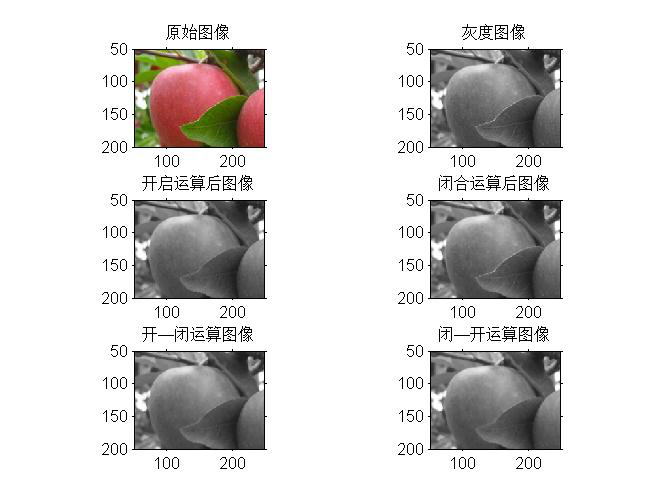
十八、开启和闭合组合操作
[plain] view plain copyfigure;  
I=imread('input_image.jpg');  
subplot(3,2,1),imshow(I);  
title('原始图像');  
axis([50,250,50,200]);  
axis on; %显示坐标系  
I1=rgb2gray(I);  
subplot(3,2,2),imshow(I1);  
title('灰度图像');  
axis([50,250,50,200]);  
axis on; %显示坐标系  
se=strel('disk',1);  
I2=imopen(I1,se); %开启操作  
I3=imclose(I1,se); %闭合操作  
subplot(3,2,3),imshow(I2);  
title('开启运算后图像');  
axis([50,250,50,200]);  
axis on; %显示坐标系  
subplot(3,2,4),imshow(I3);  
title('闭合运算后图像');  
axis([50,250,50,200]);  
axis on; %显示坐标系  
se=strel('disk',1);  
I4=imopen(I1,se);  
I5=imclose(I4,se);  
subplot(3,2,5),imshow(I5); %开—闭运算图像  
title('开—闭运算图像');  
axis([50,250,50,200]);  
axis on; %显示坐标系  
I6=imclose(I1,se);  
I7=imopen(I6,se);  
subplot(3,2,6),imshow(I7); %闭—开运算图像  
title('闭—开运算图像');  
axis([50,250,50,200]);  
axis on; %显示坐标系  
上述代码结果：



十九、形态学边界提取
[plain] view plain copyfigure;  
I=imread('input_image.jpg');  
subplot(2,3,1),imshow(I);  
title('原始图像');  
axis([50,250,50,200]);  
grid on; %显示网格线  
axis on; %显示坐标系  
I1=im2bw(I);  
subplot(2,3,2),imshow(I1);  
title('二值化图像');  
axis([50,250,50,200]);  
grid on; %显示网格线  
axis on; %显示坐标系  
   
I2=bwperim(I1); %获取区域的周长  
subplot(2,3,3),imshow(I2);  
title('边界周长的二值图像');  
axis([50,250,50,200]);  
grid on;  
axis on;  
   
I3=bwmorph(I1,'skel',1);  
subplot(2,3,4),imshow(I3);  
title('1次骨架提取');  
axis([50,250,50,200]);  
axis on;  
   
I4=bwmorph(I1,'skel',2);  
subplot(2,3,5),imshow(I4);  
title('2次骨架提取');  
axis([50,250,50,200]);  
axis on;  
上述代码结果：