吴恩达机器学习编程作业python实现--ex1

源代码使用matlab来实现，且只需要填充一些关键步骤，很容易漏掉一些信息，故而用python实现一下：

前半部分：# -*- coding: utf-8 -*-
"""
Created on Wed Mar 21 15:26:47 2018

@author: john
"""
''''
说明：本文档根据吴恩达机器学习课后作业改编而成，源代码是matlab
'''
import numpy as np
import matplotlib.pyplot as plt

def computeCost(X,y,theta):
m=len(y)
J=0
J=sum((np.dot(X,theta)-y)**2)/(2*m)
return J

def gradientDescent(X,y,theta,alpha,iterations):
m=len(y)
J_history=np.zeros((iteration,1))
for iter in range(iteration):
XT=X.T
theta=theta-alpha/m*sum(np.dot(XT,np.dot(X,theta)-y))
J_history[iter]=computeCost(X,y,theta)
return theta,J_history

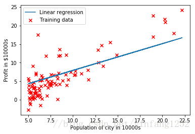
##########part1：plotting
print('Plotting Data ...\n')
data=np.loadtxt('ex1data1.txt', delimiter=',')#指定分隔符，否则会报错
X=data[:,0]
y=data[:,1]
m=len(y)#样本数
X=X.reshape((m,1))
y=y.reshape((m,1))##不reshape一下会报错

plt.figure()
plt.scatter(X,y,color='r',marker='x',linewidths=10)
plt.xlabel('Population of city in 10000s')
plt.ylabel('Profit in $10000s')
input('Program paused. Press enter to continue.\n')#调用input函数以达到暂停的目的

##########Part2: Gradient descent
X=np.concatenate((np.ones((m,1)),X),axis=1)#数组拼接
theta=np.zeros((2,1))

iteration=1500
alpha=0.01
print(computeCost(X,y,theta))
theta,J_history=gradientDescent(X,y,theta,alpha,iteration)
print('Theta found by gradient descent:')
print('%f %f \n'%( theta[0], theta[1]))
plt.plot(X[:,1],np.dot(X,theta),'-')
plt.legend(['Linear regression','Training data'])
plt.show()

predict1=np.dot(np.array([1,3.5]),theta)
predict2=np.dot(np.array([1,7]),theta)
print('For population = 35000, we predict a profit of %f\n'%(predict1[0]*10000))
#不输出[0]的话，会将原数组输出10000遍的
print('For population = 70,000, we predict a profit of %f\n'%(predict2[0]*10000))
input('Program paused. Press enter to continue.\n')

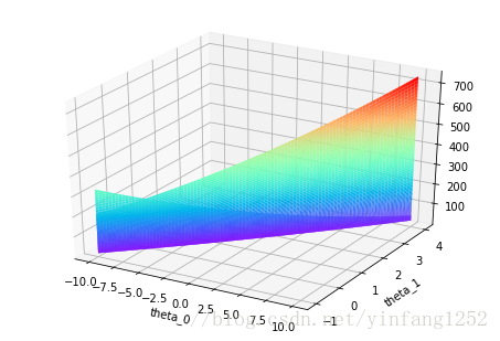
##########Part3: Visualizing J(theta_0, theta_1)
print('Visualizing J(theta_0, theta_1) ...\n')

theta0_vals = np.linspace(-10, 10, 100)
theta1_vals = np.linspace(-1, 4, 100)

J_vals = np.zeros((len(theta0_vals), len(theta1_vals)))

for i in range(len(theta0_vals)):
for j in range(len(theta1_vals)):
t=np.array([theta0_vals[i],theta1_vals[j]]).reshape((2,1))
J_vals[i,j]=computeCost(X,y,t)

J_vals=J_vals.T
from mpl_toolkits.mplot3d import Axes3D
fig = plt.figure()
ax = Axes3D(fig)
ax.plot_surface(theta0_vals,theta1_vals,J_vals,rstride=1, cstride=1, cmap='rainbow')
plt.xlabel('theta_0')
plt.ylabel('theta_1')

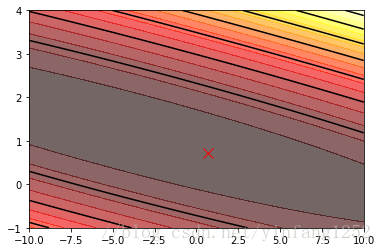
#画出等高线
plt.figure()
#填充颜色，20是等高线分为几部分
plt.contourf(theta0_vals, theta1_vals, J_vals, 20, alpha = 0.6, cmap = plt.cm.hot)
plt.contour(theta0_vals, theta1_vals, J_vals, colors = 'black')
plt.plot(theta[0], theta[1], 'r',marker='x', markerSize=10, LineWidth=2)#画点
plt.show()

结果大致如下：