【机器学习】使用Scikit-Learn库的核SVM解决非线性问题
2018-02-06 15:32
561 查看
SVM很容易的使用核技巧来解决非线性可分问题
本文使用的数据集和库文件定义在该章节有定义了,链接:http://mp.blog.csdn.net/postedit/79196206
建立异或数据集:
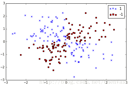
该数据集无法划分明确的边界。
核方法:通过映射函数将样本的原始特征映射到一个使样本线性可分的高维空间中。
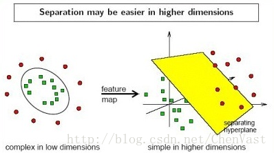
通过一个映射函数将训练集映射到高维的特征空间,并在新的空间上训练SVM,再以同样的方法应用在未知数据上。
映射方法面临的问题:构建新的特征空间带来非常大的计算成本。
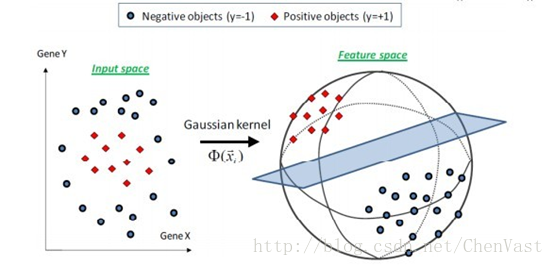
使用核函数降低两点之间的内积精确计算阶段的成本:k(xi,xj)=Φ(xi)^T Φ(xj)
应用最广泛的核函数是径向基函数或者高斯核。
公式:k(xi,xj)=exp(-y||xi-xj||^2),y=1/2σ^2
核:样本之间的“相似函数”
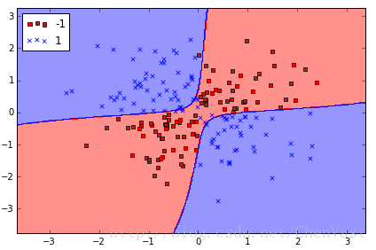
代码实现核SVM:
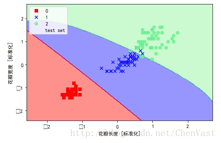
基于鸢尾花数据集的RBF核SVM:
使得类别0和1更紧凑。
本文使用的数据集和库文件定义在该章节有定义了,链接:http://mp.blog.csdn.net/postedit/79196206
建立异或数据集:
np.random.seed (0)
X_xor = np.random.randn (200, 2)
y_xor = np.logical_xor (X_xor[:, 0] > 0, X_xor[:, 1] > 0)
y_xor = np.where (y_xor, 1, -1)

plt.scatter (X_xor[y_xor == 1, 0], X_xor[y_xor == 1, 1], c='b', marker='x', label='1')
plt.scatter (X_xor[y_xor == -1, 0], X_xor[y_xor == -1, 1], c='r', marker='s', label='-1')

plt.xlim ([-3, 3])
plt.ylim ([-3, 3])
plt.legend (loc='best')
plt.tight_layout ()
# plt.savefig('./figures/xor.png', dpi=300)
plt.show ()该数据集无法划分明确的边界。
核方法:通过映射函数将样本的原始特征映射到一个使样本线性可分的高维空间中。
通过一个映射函数将训练集映射到高维的特征空间,并在新的空间上训练SVM,再以同样的方法应用在未知数据上。
映射方法面临的问题:构建新的特征空间带来非常大的计算成本。
使用核函数降低两点之间的内积精确计算阶段的成本:k(xi,xj)=Φ(xi)^T Φ(xj)
应用最广泛的核函数是径向基函数或者高斯核。
公式:k(xi,xj)=exp(-y||xi-xj||^2),y=1/2σ^2
核:样本之间的“相似函数”
代码实现核SVM:
svm = SVC(kernel='rbf', random_state=0, gamma=0.10, C=10.0)
s
4000
vm.fit(X_xor, y_xor)
plot_decision_regions(X_xor, y_xor,
classifier=svm)

plt.legend(loc='upper left')
plt.tight_layout()
# plt.savefig('./figures/support_vector_machine_rbf_xor.png', dpi=300)
plt.show()
基于鸢尾花数据集的RBF核SVM:
from sklearn.svm import SVC
svm = SVC(kernel='rbf', random_state=0, gamma=0.2, C=1.0)
svm.fit(X_train_std, y_train)
plot_decision_regions(X_combined_std, y_combined,
classifier=svm, test_idx=range(105,150))
plt.xlabel('petal length [standardized]')
plt.ylabel('petal width [standardized]')
plt.legend(loc='upper left')
plt.tight_layout()
# plt.savefig('./figures/support_vector_machine_rbf_iris_1.png', dpi=300)
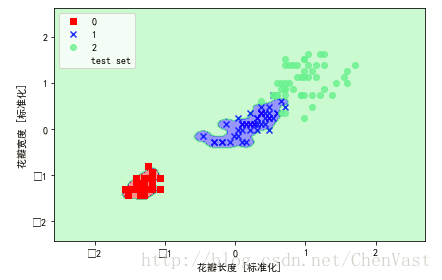
plt.show()增大gamma的值:
svm = SVC(kernel='rbf', random_state=0, gamma=100.0, C=1.0)
svm.fit(X_train_std, y_train)
plot_decision_regions(X_combined_std, y_combined,
classifier=svm, test_idx=range(105,150))
plt.xlabel('petal length [standardized]')
plt.ylabel('petal width [standardized]')
plt.legend(loc='upper left')
plt.tight_layout()
# plt.savefig('./figures/support_vector_machine_rbf_iris_2.png', dpi=300)
plt.show()使得类别0和1更紧凑。

相关文章推荐
- 【机器学习】使用Scikit-Learn库的L2正则化解决过拟合问题
- Kaggle入门——使用scikit-learn解决DigitRecognition问题
- SVM 解决类别不平衡问题(scikit_learn)
- Kaggle入门——使用scikit-learn解决DigitRecognition问题
- Kaggle入门——使用scikit-learn解决DigitRecognition问题
- 机器学习之pip安装scikit-learn问题解决
- 机器学习实战之使用 scikit-learn 库实现 svm
- Kaggle入门——使用scikit-learn解决DigitRecognition问题
- Kaggle入门——使用scikit-learn解决DigitRecognition问题
- 支持向量机之使用核SVM解决非线性分类问题
- easy.py使用中ValueError: could not convert string to float: svm_options错误问题解决
- 深度 | 解决真实世界问题:如何在不平衡类上使用机器学习?
- Python 文本分类:使用scikit-learn 机器学习包进行文本分类
- scikit-learn使用joblib.dump()持久化模型过程中的问题详解--python
- 使用scikit-learn进行机器学习的简介(教程1)
- 机器学习:scikit-learn 做笑脸识别 (SVM, KNN, Logisitc regression)
- 【机器学习实验】scikit-learn的主要模块和基本使用
- python scikit-learn 环境搭建问题解决记录
- 【机器学习实验】scikit-learn的主要模块和基本使用
- scikit-learn SVM使用和学习