An intuitive understanding of variational autoencoders without any formula
2018-02-06 10:32
495 查看
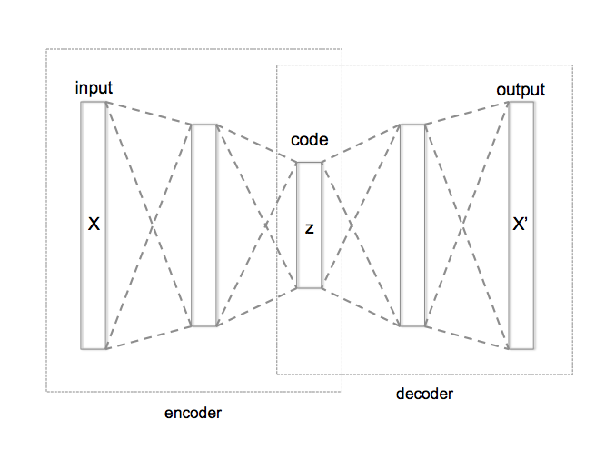
I love the simplicity of autoencoders as a very intuitive unsupervised
learning method. They are in the simplest case, a three layer neural network. In the first layer
the data comes in, the second layer typically has smaller number of nodes than the input and the third layer is similar to the input layer. These layers are usually fully connected with each other. Such networks are called auto-encoders since they first “encode”
the input to a hidden code and then “decode” it back from the hidden representation. They can be trained by simply measuring the reconstruction error and back-propagating it
to the network’s parameters. If you add noise to the input before sending it through the network, they can learn better and in that case, they are called denoising
autoencoders. They are useful because they help with understanding the data by trying to extract regularities in them and can compress them into a lower dimensional code.
A typical autoencoder can usually encode and decode data very well with low reconstruction error, but a random latent code seems to have little to do with the training data. In other words the latent code does not learn the probability distribution of the data
and therefore, if we are interested in generating more data like our dataset a typical autoencoder doesn’t seem to work as well. There is however another version of autoencoders, called “variational
autoencoder - VAE” that are able to solve this problem since they explicitly define a probability distribution on the latent code. The neural network architecture is very similar to a regular autoencoder but the difference is that the hidden code comes
from a probability distribution that is learned during the training. Since it is not very easy to navigate
through the math and equations of VAEs, I want to dedicate this post to explaining the intuition behind them. With the intuition in hand, you can understand the math and code if you want to.
I start with a short history. Over the past two decades, researchers have been trying to develop a framework for probabilistic modeling that explicitly conveys the assumption being made about the data. The result of this effort has been probabilistic
graphical models that combines ideas from graph theory and probability theory. Graphical models use a graph representation to encode a probability distribution over a set of random variables. Graph representation is a very flexible language that admit
composability for building arbitrary complex models and provides a set of tools to perform reasoning (inference) about different nodes in the graph.
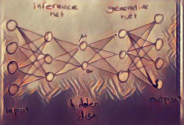
Using graphical models language we can explicitly articulate the hidden structure that we believe is generating the data. For example, if we believe that there is a hidden variable zizi for
each observable data point xixi that
is causing the data, we can make a model like this:

Since data points, XX,
are observed while the ZZ nodes
are unknown, we want to “infer” the hidden variables zizifrom
known data points. The solid line shows the data generation path and the dashed line shows the inference path.
Reasoning (inference) about hidden variables in probabilistic graphical models has traditionally been very
hard and only limited to very restricted graph structures. This issue had significantly limited our ability to build interesting models and perform reasoning on them in the past. However, in the past few years there have been some very exciting developments
that have enabled us to perform approximate reasoning with scalable algorithms like stochastic gradient descent. This has triggered another wave of interest in graphical models.
Recent developments come from the idea that directed graphical models can represent complex distributions over data while deep neural nets can represent arbitrarily complex functions. We use deep neural networks to parameterize and represent conditional distributions.
Variational autoencoders are the result of the marriage of these two set of models combined with stochastic variational and amortized inference.
A variational autoencoder is essentially a graphical model similar to the figure above in the simplest case. We assume a local latent variable, zizi for
each data point xixi.
The inference and data generation in a VAE benefit from the power of deep neural networks and scalable optimization algorithms like SGD.
As can be seen from the picture above, in a VAE, the encoder becomes a variational inference network that maps the data to the a distribution for the hidden variables, and the decoder becomes a generative network that maps the latent variables back to the data.
Since the latent variable is actually a probability distribution, we need to sample the hidden code from its distribution to be able to generate data.
In order to be able to use stochastic gradient descent with this autoencoder network, we need to be able to calculate gradients w.r.t. all the nodes in the network. However, latent variables, zz,
in a graphical model are random variables (distributions) which are not differentiable. Therefore, to make it differentiable, we treat the mean and variances of the distributions as simple deterministic parameters and multiply the variance by a sample from
a normal noise generator to add randomness. By parameterizing the hidden distribution this way, we can back-propagate the gradient to the parameters of the encoder and train the whole network with stochastic gradient descent. This procedure will allow us to
learn mean and variance values for the hidden code and it’s called the “re-parameterization
trick”. It is important to appreciate the importance of the fact that the whole network is now differentiable. This means that optimization techniques can now be used to solve the inference problem efficiently.
In classic version of neural networks we could simply measure the error of network outputs with desired target value using a simple mean
square error. But now that we are dealing with distributions, MSE is no longer a good error metric. So instead, loosely speaking, we use another metric for measuring the difference between two distributions i.e. KL-Divergence.
It turns out that this distance between our variational approximate and the real posterior distribution is not very easy to minimize either [2]. However, using some simple math, we can show that this distance is always positive and that it comprises of two
main parts (probability of data minus a function called ELBO). So instead of minimizing the whole thing, we can maximize the smaller term (ELBO) [4]. This term comes from marginalizing the log-probability of data and is always smaller than the log probability
of the data. That’s why we call it a lower bound on the evidence (data given model). From the perspective of autoencoders, the ELBO function can be seen as the sum of the reconstruction cost of the input plus the regularization terms.
If after maximizing the ELBO, the lower bound of data is close to the data distribution, then the distance is close to zero and voila!; We have minimized the error distance indirectly. The algorithm we use to maximize the lower bound is the exact opposite of
gradient descent. Instead of going in the reverse direction of the gradient to get to the minimum, we go toward the positive direction to get to the maximum, so it’s now called gradient ascent! This whole algorithm is called “autoencoding variational Bayes”
[1]! After we are done with the learning we can visualize the latent space of our VAE and generate samples from it. Pretty cool, eh!?
Here is a high level pseudo-code for the architecture of a VAE to put things into perspective:
Now that the intuition is clear, here is a Jupyter notebook for playing with VAEs,
if you like to learn more. The notebook is based on this Keras example. The
resulting learned latent space of the encoder and the manifold of a simple VAE trained on the MNIST dataset are below.
Side note 1:
The ELBO is determined from introducing a variational distribution q, on lower bound on the marginal log likelihood, i.e. log p(x)=log∫zp(x,z)∗q(z|x)q(z|x)log p(x)=log∫zp(x,z)∗q(z|x)q(z|x).
We use the log likelihood to be able to use the concavity of the loglog function
and employ Jensen’s equation to move the loglog inside
the integral i.e. log p(x)>∫zlog (p(x,z)∗q(z|x)q(z|x))log p(x)>∫zlog (p(x,z)∗q(z|x)q(z|x)) and
then use the definition of expectation on qq (the
nominator qq goes
into the definition of the expectation on qq to
write that as the ELBO) log p(x)>ELBO(z)=Eq[−log q(z|x)+log p(x,z)]log p(x)>ELBO(z)=Eq[−log q(z|x)+log p(x,z)].
The difference between the ELBO and the marginal p(x)p(x) which
converts the inequality to an equality is the distance between the real posterior and the approximate posterior i.e. KL[q(z|x) | p(z|x)]KL[q(z|x) | p(z|x)].
Alternatively, the distance between the ELBO and the KL term is the log-normalizer p(x)p(x).
Replace the p(z|x)p(z|x) with
Bayesian formula to see how.
Now that we have a defined a loss function, we need the gradient of the loss function, δEq[−logq(z|x)+p(x,z)]δEq[−logq(z|x)+p(x,z)] to
be able to use it for optimization with SGD. The gradient isn’t easy to derive analytically but we can estimate it by using MCMC to directly sample from q(z|x)q(z|x) and
estimate the gradient. This approach generally exhibits large variance since MCMC might sample from rare values.
This is where the re-parameterization trick we discussed above comes in. We assume that the random variable zzis
a deterministic function of xx and
a known ϵϵ (ϵϵ are
iid samples) that injects randomness z=g(x,ϵ)z=g(x,ϵ).
This re-parameterization converts the undifferentiable random variable zz,
to a differentiable function of xx and
a decoupled source of randomness. Therefore, using this re-parameterization, we can estimate the gradient of the ELBO as δEϵ[δ−log q(g(x,ϵ)|x)+δp(x,g(x,ϵ))]δEϵ[δ−log q(g(x,ϵ)|x)+δp(x,g(x,ϵ))].
This estimate to the gradient has empirically shown to have much less variance and is called “Stochastic Gradient Variational Bayes (SGVB)”. The SGVB is also called a black-box inference method (similar to MCMC estimate of the gradient) which simply means
it doesn’t care what functions we use in the generative and inference network. It only needs to be able the calculate the gradient at samples of ϵϵ.
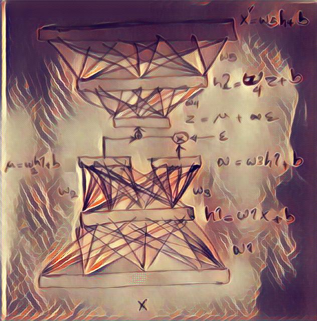
We can use SGVB with a separate set of parameters for each observation however that’s costly and inefficient. We usually choose to “amortize” the cost of inference with deep networks (to learn a single complex function for all observations instead). All the
terms of the ELBO are differentiable now if we choose deep networks as our likelihood and approximate posterior functions. Therefore, we have an end-to-end differentiable model. Following depiction shows amortized SGVB re-parameterization in a VAE.
side note 2:
Note that in the above derivation of the ELBO, the first term is the entropy of the variational posterior and second term is log of joint distribution. However we usually write joint distribution as p(x,z)=p(x|z)p(z)p(x,z)=p(x|z)p(z) to
rewrite the ELBO as Eq[log p(x|z)+KL(q(z|x) | p(z))]Eq[log p(x|z)+KL(q(z|x) | p(z))].
This derivation is much closer to the typical machine learning literature in deep networks. The first term is log likelihood (i.e. reconstruction cost) while the second term is KL divergence between the prior and the posterior (i.e a regularization term that
won’t allow posterior to deviate much from the prior). Also note that if we only use the first term as our cost function, the learning with correspond to maximum likelihood learning that does not include regularization and might overfit.
Side note 3: problems that we might encounter while working with VAE;
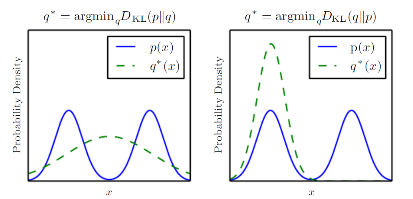
It’s useful to think about the distance measure we talked about. KL-divergence measures a sort of distance between two distributions but it’s not a true distance since it’s not symmetricKL(P|Q)=EP[log P(x)−log Q(x)]KL(P|Q)=EP[log P(x)−log Q(x)].
So which distance direction we choose to minimize has consequences. For example, in minimizing KL(p|q)KL(p|q),
we select a qq that
has high probability where pp has
high probability so when pp has
multiple modes, qq chooses
to blur the modes together, in order to put high probability mass on all of them.
On the other hand, in minimizing KL(q|p)KL(q|p),
we select a qq that
has low probability where pp has
low probability. When pp has
multiple modes that are sufficiently widely separated, the KL divergence is minimized by choosing a single mode (mode collapsing), in order to avoid putting probability mass in the low-probability areas between modes of pp.
In VAEs we actually minimize KL(q|p)KL(q|p) so
mode collapsing is a common problem. Additionally, due to the complexity of true distributions we also see blurring problem. These two cases are illustrated in the following figure from the deep
learning book.
references:
[1] Kingma, Diederik P., and Max Welling. “Auto-encoding variational Bayes.” arXiv preprint arXiv:1312.6114 (2013).
[2] Rezende, Danilo Jimenez, Shakir Mohamed, and Daan Wierstra. “Stochastic backpropagation and approximate inference in deep generative models.” arXiv preprint arXiv:1401.4082 (2014).
[3] https://www.cs.princeton.edu/courses/archive/fall11/cos597C/lectures/variational-inference-i.pdf
原文地址: https://hsaghir.github.io/data_science/denoising-vs-variational-autoencoder/
learning method. They are in the simplest case, a three layer neural network. In the first layer
the data comes in, the second layer typically has smaller number of nodes than the input and the third layer is similar to the input layer. These layers are usually fully connected with each other. Such networks are called auto-encoders since they first “encode”
the input to a hidden code and then “decode” it back from the hidden representation. They can be trained by simply measuring the reconstruction error and back-propagating it
to the network’s parameters. If you add noise to the input before sending it through the network, they can learn better and in that case, they are called denoising
autoencoders. They are useful because they help with understanding the data by trying to extract regularities in them and can compress them into a lower dimensional code.
A typical autoencoder can usually encode and decode data very well with low reconstruction error, but a random latent code seems to have little to do with the training data. In other words the latent code does not learn the probability distribution of the data
and therefore, if we are interested in generating more data like our dataset a typical autoencoder doesn’t seem to work as well. There is however another version of autoencoders, called “variational
autoencoder - VAE” that are able to solve this problem since they explicitly define a probability distribution on the latent code. The neural network architecture is very similar to a regular autoencoder but the difference is that the hidden code comes
from a probability distribution that is learned during the training. Since it is not very easy to navigate
through the math and equations of VAEs, I want to dedicate this post to explaining the intuition behind them. With the intuition in hand, you can understand the math and code if you want to.
I start with a short history. Over the past two decades, researchers have been trying to develop a framework for probabilistic modeling that explicitly conveys the assumption being made about the data. The result of this effort has been probabilistic
graphical models that combines ideas from graph theory and probability theory. Graphical models use a graph representation to encode a probability distribution over a set of random variables. Graph representation is a very flexible language that admit
composability for building arbitrary complex models and provides a set of tools to perform reasoning (inference) about different nodes in the graph.
Using graphical models language we can explicitly articulate the hidden structure that we believe is generating the data. For example, if we believe that there is a hidden variable zizi for
each observable data point xixi that
is causing the data, we can make a model like this:
Since data points, XX,
are observed while the ZZ nodes
are unknown, we want to “infer” the hidden variables zizifrom
known data points. The solid line shows the data generation path and the dashed line shows the inference path.
Reasoning (inference) about hidden variables in probabilistic graphical models has traditionally been very
hard and only limited to very restricted graph structures. This issue had significantly limited our ability to build interesting models and perform reasoning on them in the past. However, in the past few years there have been some very exciting developments
that have enabled us to perform approximate reasoning with scalable algorithms like stochastic gradient descent. This has triggered another wave of interest in graphical models.
Recent developments come from the idea that directed graphical models can represent complex distributions over data while deep neural nets can represent arbitrarily complex functions. We use deep neural networks to parameterize and represent conditional distributions.
Variational autoencoders are the result of the marriage of these two set of models combined with stochastic variational and amortized inference.
A variational autoencoder is essentially a graphical model similar to the figure above in the simplest case. We assume a local latent variable, zizi for
each data point xixi.
The inference and data generation in a VAE benefit from the power of deep neural networks and scalable optimization algorithms like SGD.
As can be seen from the picture above, in a VAE, the encoder becomes a variational inference network that maps the data to the a distribution for the hidden variables, and the decoder becomes a generative network that maps the latent variables back to the data.
Since the latent variable is actually a probability distribution, we need to sample the hidden code from its distribution to be able to generate data.
In order to be able to use stochastic gradient descent with this autoencoder network, we need to be able to calculate gradients w.r.t. all the nodes in the network. However, latent variables, zz,
in a graphical model are random variables (distributions) which are not differentiable. Therefore, to make it differentiable, we treat the mean and variances of the distributions as simple deterministic parameters and multiply the variance by a sample from
a normal noise generator to add randomness. By parameterizing the hidden distribution this way, we can back-propagate the gradient to the parameters of the encoder and train the whole network with stochastic gradient descent. This procedure will allow us to
learn mean and variance values for the hidden code and it’s called the “re-parameterization
trick”. It is important to appreciate the importance of the fact that the whole network is now differentiable. This means that optimization techniques can now be used to solve the inference problem efficiently.
In classic version of neural networks we could simply measure the error of network outputs with desired target value using a simple mean
square error. But now that we are dealing with distributions, MSE is no longer a good error metric. So instead, loosely speaking, we use another metric for measuring the difference between two distributions i.e. KL-Divergence.
It turns out that this distance between our variational approximate and the real posterior distribution is not very easy to minimize either [2]. However, using some simple math, we can show that this distance is always positive and that it comprises of two
main parts (probability of data minus a function called ELBO). So instead of minimizing the whole thing, we can maximize the smaller term (ELBO) [4]. This term comes from marginalizing the log-probability of data and is always smaller than the log probability
of the data. That’s why we call it a lower bound on the evidence (data given model). From the perspective of autoencoders, the ELBO function can be seen as the sum of the reconstruction cost of the input plus the regularization terms.
If after maximizing the ELBO, the lower bound of data is close to the data distribution, then the distance is close to zero and voila!; We have minimized the error distance indirectly. The algorithm we use to maximize the lower bound is the exact opposite of
gradient descent. Instead of going in the reverse direction of the gradient to get to the minimum, we go toward the positive direction to get to the maximum, so it’s now called gradient ascent! This whole algorithm is called “autoencoding variational Bayes”
[1]! After we are done with the learning we can visualize the latent space of our VAE and generate samples from it. Pretty cool, eh!?
Here is a high level pseudo-code for the architecture of a VAE to put things into perspective:
network= {

# encoder
encoder_x = Input_layer(size=input_size, input=data)
encoder_h = Dense_layer(size=hidden_size, input= encoder_x)

# the re-parameterized distributions that are inferred from data
z_mean = Dense(size=number_of_distributions, input=encoder_h)
z_variance = Dense(size=number_of_distributions, input=encoder_h)
epsilon= random(size=number_of_distributions)

# decoder network needs a sample from the code distribution
z_sample= z_mean + exp(z_variance / 2) * epsilon

#decoder
decoder_h = Dense_layer(size=hidden_size, input=z_sample)
decoder_output = Dense_layer(size=input_size, input=decoder_h)
}

cost={
reconstruction_loss = input_size * crossentropy(data, decoder_output)
kl_loss = - 0.5 * sum(1 + z_variance - square(z_mean) - exp(z_variance))
cost_total= reconstruction_loss + kl_loss
}

stochastic_gradient_descent(data, network, cost_total)
Now that the intuition is clear, here is a Jupyter notebook for playing with VAEs,
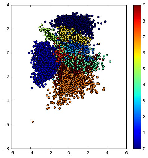
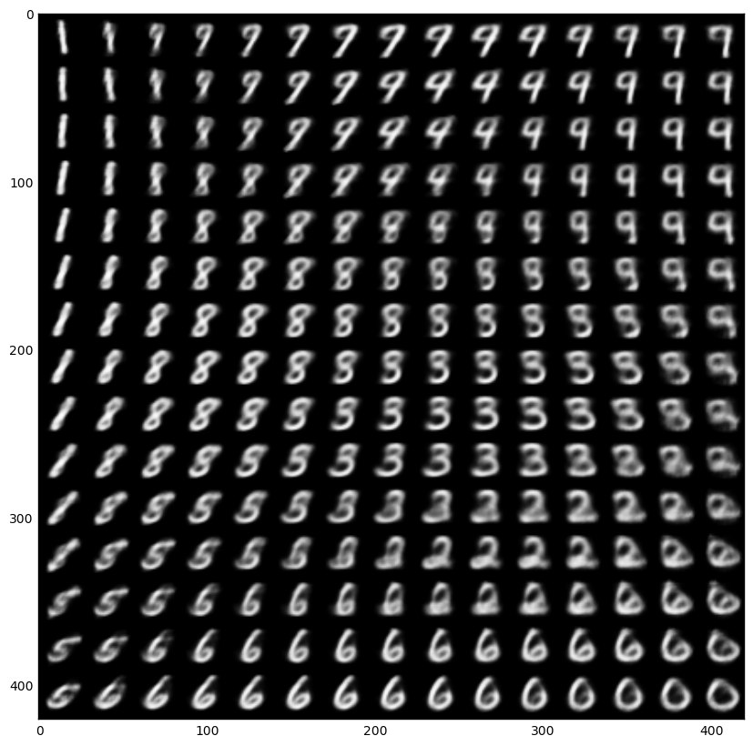
if you like to learn more. The notebook is based on this Keras example. The
resulting learned latent space of the encoder and the manifold of a simple VAE trained on the MNIST dataset are below.
 |  |
Side note 1:
The ELBO is determined from introducing a variational distribution q, on lower bound on the marginal log likelihood, i.e. log p(x)=log∫zp(x,z)∗q(z|x)q(z|x)log p(x)=log∫zp(x,z)∗q(z|x)q(z|x).
We use the log likelihood to be able to use the concavity of the loglog function
and employ Jensen’s equation to move the loglog inside
the integral i.e. log p(x)>∫zlog (p(x,z)∗q(z|x)q(z|x))log p(x)>∫zlog (p(x,z)∗q(z|x)q(z|x)) and
then use the definition of expectation on qq (the
nominator qq goes
into the definition of the expectation on qq to
write that as the ELBO) log p(x)>ELBO(z)=Eq[−log q(z|x)+log p(x,z)]log p(x)>ELBO(z)=Eq[−log q(z|x)+log p(x,z)].
The difference between the ELBO and the marginal p(x)p(x) which
converts the inequality to an equality is the distance between the real posterior and the approximate posterior i.e. KL[q(z|x) | p(z|x)]KL[q(z|x) | p(z|x)].
Alternatively, the distance between the ELBO and the KL term is the log-normalizer p(x)p(x).
Replace the p(z|x)p(z|x) with
Bayesian formula to see how.
Now that we have a defined a loss function, we need the gradient of the loss function, δEq[−logq(z|x)+p(x,z)]δEq[−logq(z|x)+p(x,z)] to
be able to use it for optimization with SGD. The gradient isn’t easy to derive analytically but we can estimate it by using MCMC to directly sample from q(z|x)q(z|x) and
estimate the gradient. This approach generally exhibits large variance since MCMC might sample from rare values.
This is where the re-parameterization trick we discussed above comes in. We assume that the random variable zzis
a deterministic function of xx and
a known ϵϵ (ϵϵ are
iid samples) that injects randomness z=g(x,ϵ)z=g(x,ϵ).
This re-parameterization converts the undifferentiable random variable zz,
to a differentiable function of xx and
a decoupled source of randomness. Therefore, using this re-parameterization, we can estimate the gradient of the ELBO as δEϵ[δ−log q(g(x,ϵ)|x)+δp(x,g(x,ϵ))]δEϵ[δ−log q(g(x,ϵ)|x)+δp(x,g(x,ϵ))].
This estimate to the gradient has empirically shown to have much less variance and is called “Stochastic Gradient Variational Bayes (SGVB)”. The SGVB is also called a black-box inference method (similar to MCMC estimate of the gradient) which simply means
it doesn’t care what functions we use in the generative and inference network. It only needs to be able the calculate the gradient at samples of ϵϵ.
We can use SGVB with a separate set of parameters for each observation however that’s costly and inefficient. We usually choose to “amortize” the cost of inference with deep networks (to learn a single complex function for all observations instead). All the
terms of the ELBO are differentiable now if we choose deep networks as our likelihood and approximate posterior functions. Therefore, we have an end-to-end differentiable model. Following depiction shows amortized SGVB re-parameterization in a VAE.
side note 2:
Note that in the above derivation of the ELBO, the first term is the entropy of the variational posterior and second term is log of joint distribution. However we usually write joint distribution as p(x,z)=p(x|z)p(z)p(x,z)=p(x|z)p(z) to
rewrite the ELBO as Eq[log p(x|z)+KL(q(z|x) | p(z))]Eq[log p(x|z)+KL(q(z|x) | p(z))].
This derivation is much closer to the typical machine learning literature in deep networks. The first term is log likelihood (i.e. reconstruction cost) while the second term is KL divergence between the prior and the posterior (i.e a regularization term that
won’t allow posterior to deviate much from the prior). Also note that if we only use the first term as our cost function, the learning with correspond to maximum likelihood learning that does not include regularization and might overfit.
Side note 3: problems that we might encounter while working with VAE;
It’s useful to think about the distance measure we talked about. KL-divergence measures a sort of distance between two distributions but it’s not a true distance since it’s not symmetricKL(P|Q)=EP[log P(x)−log Q(x)]KL(P|Q)=EP[log P(x)−log Q(x)].
So which distance direction we choose to minimize has consequences. For example, in minimizing KL(p|q)KL(p|q),
we select a qq that
has high probability where pp has
high probability so when pp has
multiple modes, qq chooses
to blur the modes together, in order to put high probability mass on all of them.
On the other hand, in minimizing KL(q|p)KL(q|p),
we select a qq that
has low probability where pp has
low probability. When pp has
multiple modes that are sufficiently widely separated, the KL divergence is minimized by choosing a single mode (mode collapsing), in order to avoid putting probability mass in the low-probability areas between modes of pp.
In VAEs we actually minimize KL(q|p)KL(q|p) so
mode collapsing is a common problem. Additionally, due to the complexity of true distributions we also see blurring problem. These two cases are illustrated in the following figure from the deep
learning book.
references:
[1] Kingma, Diederik P., and Max Welling. “Auto-encoding variational Bayes.” arXiv preprint arXiv:1312.6114 (2013).
[2] Rezende, Danilo Jimenez, Shakir Mohamed, and Daan Wierstra. “Stochastic backpropagation and approximate inference in deep generative models.” arXiv preprint arXiv:1401.4082 (2014).
[3] https://www.cs.princeton.edu/courses/archive/fall11/cos597C/lectures/variational-inference-i.pdf
原文地址: https://hsaghir.github.io/data_science/denoising-vs-variational-autoencoder/

相关文章推荐
- Exception: Operation xx of contract xx specifies multiple request body parameters to be serialized without any wrapper elements.
- An Intuitive Explanation of Convolutional Neural Networks
- an example of using automake.
- Implicit conversion of an Objective-C pointer to '__autoreleasing instancetype *' (aka '__autoreleas
- Tutorial on Variational AutoEncoders
- Semi-supervised Segmentation of Optic Cup in Retinal Fundus Images Using Variational Autoencoder 论文笔记
- A wizard’s guide to Adversarial Autoencoders: Part 3, Disentanglement of style and content.
- Auto Memory Dump on Crash of an Application
- An Intuitive Explanation of Convolutional Neural Networks
- How do you copy the contents of an array to a std::vector in C++ without looping? (From stack over flow)
- An Intuitive Explanation of Convolutional Neural Networks
- Variational AutoEncoders(VAE)
- ios implicit conversion of an objective-c pointer to 'NSString *__autoreleasing *' is disallowed wit
- Understanding Windows CardSpace: An Introduction to the Concepts and Challenges of Digital Identitie
- An Intuitive Explanation of Convolutional Neural Networks
- When using SqlDependency without providing an options value, SqlDependency.Start() must be called prior to execution of a command added to the SqlDependency instance.
- Becoming an Xperf Xpert Part 3: The Case of When Auto “wait for it” Logon is Slow
- 一个直观的图像傅里叶实例(An Intuitive Explanation of Fourier Theory)
- Given an array of size N in which every number is between 1 and N, determine if there are any dupli
- Flipping Bits in Memory Without Accessing Them: An Experimental Study of DRAM Disturbance Errors