用Python研究了三千套房子，告诉你究竟是什么抬高了房价？（python实战）

https://www.tuicool.com/articles/FBvaM3f

关于房价，一直都是全民热议的话题，毕竟不少人终其一生都在为之奋斗。

房地产的泡沫究竟有多大不得而知？今天我们抛开泡沫，回归房屋最本质的内容，来分析一下房价的影响因素究竟是什么？

1、导入数据

import numpy as np 
 
import pandas as pd 
 
import matplotlib.pyplot as plt 
 
import seaborn as sn 
 
import missingno as msno 
 
%matplotlib inline 
 
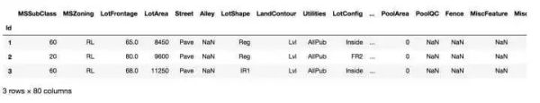
train = pd.read_csv('train.csv',index_col=0)  
 
#导入训练集 
 
test = pd.read_csv('test.csv',index_col=0)  
 
#导入测试集 
 
train.head(3) 
 
print('train训练集缺失数据分布图') 
 
msno.matrix(train) 
 
print('test测试集缺失数据分布图') 
 
msno.matrix(test) 







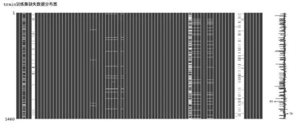
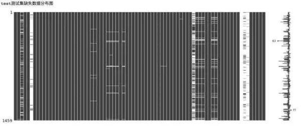
从上面的数据缺失可视化图中可以看出，部分特征的数据缺失十分严重，下面我们来对特征的缺失数量进行统计。

2、目标Y值分析

##分割Y和X数据 
 
y=train['SalePrice'] 
 
#看一下y的值分布 
 
prices = pd.DataFrame({'price':y,'log(price+1)':np.log1p(y)}) 
 
prices.hist() 



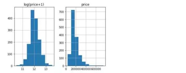
观察目标变量y的分布和取对数后的分布看，取完对数后更倾向于符合正太分布，故我们对y进行对数转化。

y = np.log1p(y) #+1的目的是防止对数转化后的值无意义 

3、合并数据 缺失处理

#合并训练特征和测试集 
 
all_df = pd.concat((X,test),axis=0) 
 
print('all_df缺失数据图') 
 
msno.matrix(all_df) 
 
#定义缺失统计函数 
 
def show_missing(feature): 
 
    missing = feature.columns[feature.isnull().any()].tolist()     
 
return  missing 
 
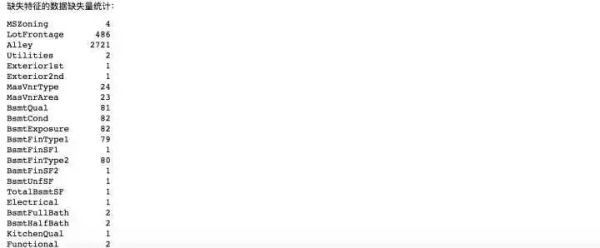
print('缺失特征的数据缺失量统计：') 
 
all_df[show_missing(all_df)].isnull().sum() 
 
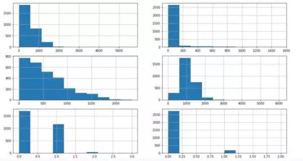
#先处理numeric数值型数据 
 
#挨个儿看一下分布 
 
fig,axs = plt.subplots(3,2,figsize=(16,9)) 
 
all_df['BsmtFinSF1'].hist(ax = axs[0,0])#众数填充 
 
all_df['BsmtFinSF2'].hist(ax = axs[0,1])#众数 
 
all_df['BsmtUnfSF'].hist(ax =  axs[1,0])#中位数 
 
all_df['TotalBsmtSF'].hist(ax = axs[1,1])#均值填充 
 
all_df['BsmtFullBath'].hist(ax = axs[2,0])#众数 
 
all_df['BsmtHalfBath'].hist(ax = axs[2,1])#众数 
 
#lotfrontage用均值填充 
 
mean_lotfrontage = all_df.LotFrontage.mean() 
 
all_df.LotFrontage.hist() 
 
print('用均值填充:') 
 
cat_input(all_df,'LotFrontage',mean_lotfrontage) 
 
cat_input(all_df,'BsmtFinSF1',0.0) 
 
cat_input(all_df,'BsmtFinSF2',0.0) 
 
cat_input(all_df,'BsmtFullBath',0.0) 
 
cat_input(all_df,'BsmtHalfBath',0.0) 
 
cat_input(all_df,'BsmtUnfSF',467.00) 
 
cat_input(all_df,'TotalBsmtSF',1051.78) 
 
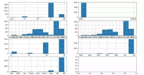
#在处理字符型，同样，挨个看下分布 
 
fig,axs = plt.subplots(4,2,figsize=(16,9)) 
 
all_df['MSZoning'].hist(ax = axs[0,0])#众数填充 
 
all_df['Utilities'].hist(ax = axs[0,1])#众数 
 
all_df['Exterior1st'].hist(ax =  axs[1,0])#众数 
 
all_df['Exterior2nd'].hist(ax = axs[1,1])#众数填充 
 
all_df['KitchenQual'].hist(ax = axs[2,0])#众数 
 
all_df['Functional'].hist(ax = axs[2,1])#众数 
 
all_df['SaleType'].hist(ax = axs[3,0])#众数 
 
cat_input(all_df,'MSZoning','RL') 
 
cat_input(all_df,'Utilities','AllPub') 
 
cat_input(all_df,'Exterior1st','VinylSd') 
 
cat_input(all_df,'Exterior2nd','VinylSd') 
 
cat_input(all_df,'KitchenQual','TA') 
 
cat_input(all_df,'Functional','Typ') 
 
cat_input(all_df,'SaleType','WD') 
 
#再看一下缺失分布 
 
msno.matrix(all_df) 











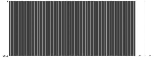
binggo，数据干净啦！下面开始处理特征,经过上述略微复杂的处理，数据集中所有的缺失数据都已处理完毕，可以开始接下来的工作啦！

缺失处理总结：在本篇文章所使用的数据集中存在比较多的缺失，缺失数据包括数值型和字符型，处理原则主要有两个：

一、根据绘制数据分布直方图，观察数据分布的状态，采取合适的方式填充缺失数据；

二、非常重要的特征描述，认真阅读，按照特征描述填充可以解决大部分问题。

4、特征处理

让我们在重新仔细审视一下数据有没有问题？仔细观察发现MSSubClass特征实际上是分类特征，但是数据显示是int类型，这个需要改成str。

#观察特征属性发现，MSSubClass是分类特征，但是数据给的是数值型，需要对其做转换 
 
all_df['MSSubClass']=all_df['MSSubClass'].astype(str) 
 
#将分类变量转变成数值变量 
 
all_df = pd.get_dummies(all_df) 
 
print('分类变量转换完成后有{}行{}列'.format(*all_df.shape))  

分类变量转换完成后有2919行316列

#标准化处理 
 
numeric_cols = all_df.columns[all_df.dtypes !='uint8'] 
 
#x-mean(x)/std(x) 
 
numeric_mean = all_df.loc[:,numeric_cols].mean() 
 
numeric_std = all_df.loc[:,numeric_cols].std() 
 
all_df.loc[:,numeric_cols] = (all_df.loc[:,numeric_cols]-numeric_mean)/numeric_std  

再把数据拆分到训练集和测试集

train_df = all_df.ix[0:1460]#训练集 
 
test_df = all_df.ix[1461:]#测试集  

5、构建基准模型

from sklearn import cross_validation 
 
from sklearn import linear_model 
 
from sklearn.learning_curve import learning_curve 
 
from sklearn.metrics import explained_variance_score 
 
from sklearn.grid_search import GridSearchCV 
 
from sklearn.model_selection import cross_val_score 
 
from sklearn.ensemble import RandomForestRegressor 
 
y = y.values #转换成array数组 
 
X = train_df.values #转换成array数组 
 
cv = cross_validation.ShuffleSplit(len(X),n_iter=3,test_size=0.2) 
 
print('岭回归交叉验证结果：') 
 
for train_index,test_index in cv: 
 
    ridge = linear_model.Ridge(alpha=1).fit(X,y)     
 
   print('train_score:{0:.3f},test_score:{1:.3f}\n'.format(ridge.score(X[train_index],y[train_index]), ridge.score(X[test_index],y[test_index]))) 
 
print('随机森林交叉验证结果：') 
 
for train_index,test_index in cv: 
 
    rf = RandomForestRegressor().fit(X,y)     
 
    print('train_score:{0:.3f},test_score:{1:.3f}\n'.format(rf.score(X[train_index],y[train_index]), rf.score(X[test_index],y[test_index]))) 



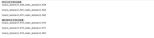
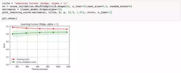
哇！好意外啊，这两个模型的结果表现都不错，但是随机森林的结果似乎更好，下面来看看学习曲线情况。





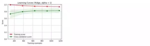
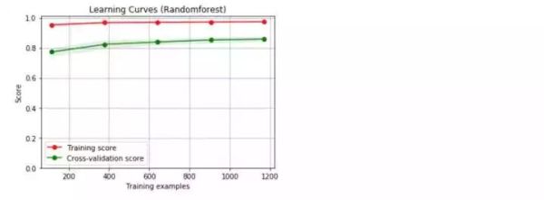
我们采用的是默认的参数，没有调优处理，得到的两个基准模型都存在过拟合现象。下面，我们开始着手参数的调整，希望能够改善模型的过拟合现象。

6、参数调优

岭回归正则项缩放系数alpha调整

alphas =[0.01,0.1,1,10,20,50,100,300] 
 
test_scores = [] 
 
for alp in alphas: 
 
    clf = linear_model.Ridge(alp) 
 
    test_score = -cross_val_score(clf,X,y,cv=10,scoring='neg_mean_squared_error') 
 
    test_scores.append(np.mean(test_score)) 
 
import matplotlib.pyplot as plt 
 
%matplotlib inline 
 
plt.plot(alphas,test_scores) 
 
plt.title('alpha vs test_score') 



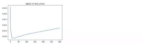
alpha在10-20附近均方误差最小

随机森林参数调优

随机森林算法，本篇中主要调整三个参数：maxfeatures,maxdepth,n_estimators

#随机森林的深度参数 
 
max_depth=[2,4,6,8,10] 
 
test_scores_depth = [] 
 
for depth in max_depth: 
 
    clf = RandomForestRegressor(max_depth=depth) 
 
    test_score_depth = -cross_val_score(clf,X,y,cv=10,scoring='neg_mean_squared_error') 
 
    test_scores_depth.append(np.mean(test_score_depth)) 
 
#随机森林的特征个数参数 
 
max_features =[.1, .3, .5, .7, .9, .99] 
 
test_scores_feature = [] 
 
for feature in max_features: 
 
    clf = RandomForestRegressor(max_features=feature) 
 
    test_score_feature = -cross_val_score(clf,X,y,cv=10,scoring='neg_mean_squared_error') 
 
    test_scores_feature.append(np.mean(test_score_feature)) 
 
#随机森林的估计器个位数参数 
 
n_estimators =[10,50,100,200,500] 
 
test_scores_n = [] 
 
for n in n_estimators: 
 
    clf = RandomForestRegressor(n_estimators=n) 
 
    test_score_n = -cross_val_score(clf,X,y,cv=10,scoring='neg_mean_squared_error') 
 
    test_scores_n.append(np.mean(test_score_n)) 







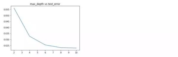
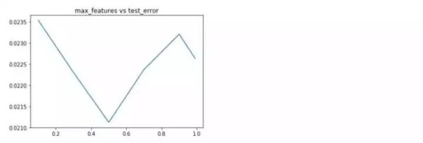
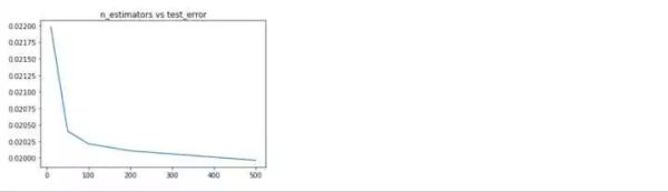
随机森林的各项参数来看，深度位于8，选择特征个数比例为0.5，估计器个数为500时，效果最好。下面分别利用上述得到的最优参数分别重新训练，看一下学习曲线，过拟合现象是否得到缓解？





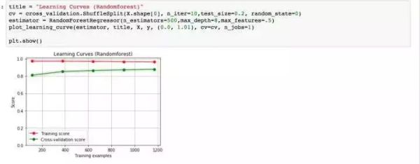
再回想一下，我们最初的基线模型学习曲线的形状，是不是得到了一定程度的缓解？OK，下面我们采用模型融合技术，对数据进行预测。

#预测 
 
ridge = linear_model.Ridge(alpha=10).fit(X,y) 
 
rf = RandomForestRegressor(n_estimators=500,max_depth=8,max_features=.5).fit(X,y) 
 
y_ridge = np.expm1(ridge.predict(test_df.values)) 
 
y_rf = np.expm1(rf.predict(test_df.values)) 
 
y_final = (y_ridge + y_rf)/2 



本篇房价预测的模型搭建已经完成。同样，再梳理一边思路：

一、本篇用到的房价数据集存在比较多的数据缺失，且分类变量十分多。在预处理阶段需要将训练集和测试集合并，进行缺失填充和one-hot独热变量处理，保证数据处理过程的一致性，在数据缺失填充过程中，需要综合考虑特征的实际描述和数据的分布，选择合适的填充方式填充；

二、为防止数据变量不统一带来的模型准确率下降，将数值型特征进行标准化处理，数据处理完成后，按照数据合并的方式，再还原到训练集和测试集；

三、先构建岭回归和随机森林基准模型，进行三折交叉验证，绘制学习曲线，存在明显的过拟合现象；

四、接下来分别对两个基准模型进行参数调优，获得使得均方误差最小的参数，返回到训练集进行训练；

五、采用并行模型融合的方式，计算两个模型预测结果的均值作为测试集的预测结果。