[DL]2.使用Softmax回归进行手写数字识别
2017-08-19 00:48
447 查看
本文对TensorFlow官方示例-手写数字识别教程的读书笔记。
教程分为3个部分:
数据准备
模型建立
模型评价
这里需要注意的是,数据集中保存的并不是真正的一张张真实的图片,而是用矩阵对数据进行了展示。比如,训练记中的数据表示为:

它是一个55000×784维的张量,表示有55000张图片,每张图片用784维的一维向量表示。
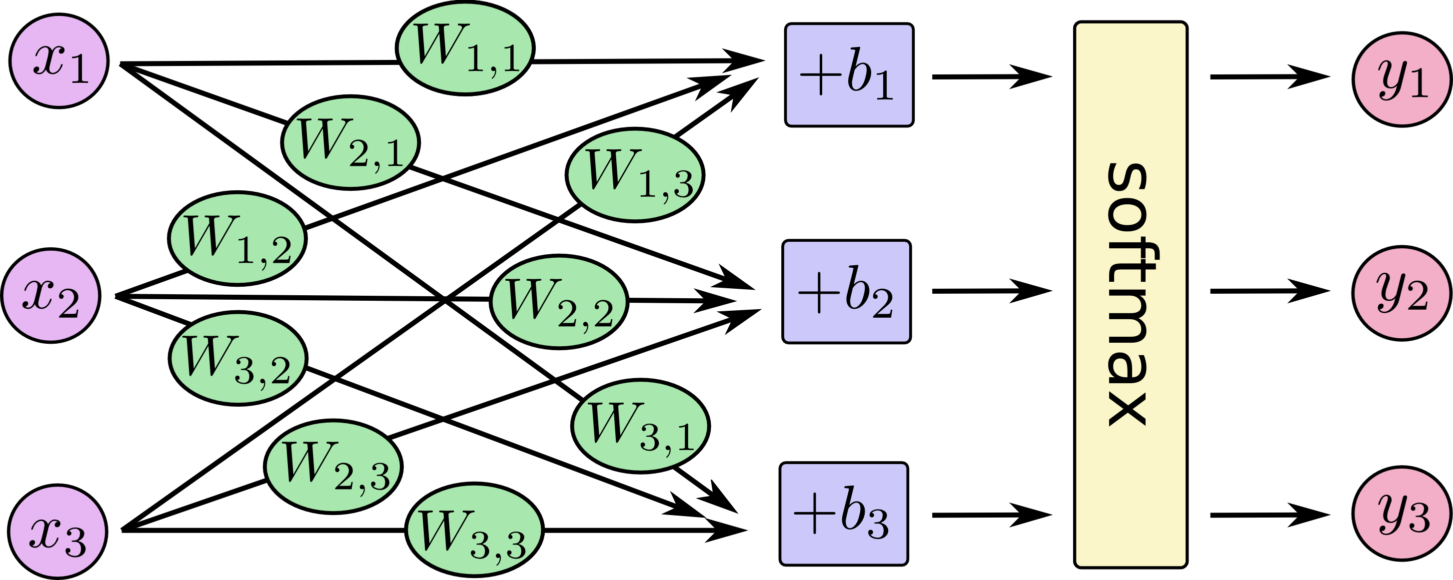
x是向量形式的图片,w表示每一个像素的权重,b表示偏置值。yi表示为第i个数字的置信度。
用公式表示为:
y=softmax(Wx+b)
损失函数定义为:
Hy′(y)=−∑iy′ilog(yi)
其中y′是真实值,y是预测值。训练的目标就是使得Hy′(y)最小。
下面结合代码进行解释:
教程分为3个部分:
数据准备
模型建立
模型评价
1.数据准备
教程使用的是公开的MNIST手写数字图片记,并且对数据的访问进行了封装,因此在实际编码过程中很方便的就可以将数据准备好。这里需要注意的是,数据集中保存的并不是真正的一张张真实的图片,而是用矩阵对数据进行了展示。比如,训练记中的数据表示为:
它是一个55000×784维的张量,表示有55000张图片,每张图片用784维的一维向量表示。
2.模型建立
本教程使用的模型可以直观的表示为:x是向量形式的图片,w表示每一个像素的权重,b表示偏置值。yi表示为第i个数字的置信度。
用公式表示为:
y=softmax(Wx+b)
损失函数定义为:
Hy′(y)=−∑iy′ilog(yi)
其中y′是真实值,y是预测值。训练的目标就是使得Hy′(y)最小。
下面结合代码进行解释:
from tensorflow.examples.tutorials.mnist import input_data

print('数据加载...')
mnist=input_data.read_data_sets('./data/mnist',one_hot=True)
# 可以看到返回的是Datasets类型,包含了训练集、验证集、测试集
#return base.Datasets(train=train, validation=validation, test=test)

print('图片表示示例:')
print(mnist[0].images[0])
print('标签表示示例:')
print(mnist[0].labels[0])

img_count_train=len(mnist[0].images)
img_array_train=len(mnist[0].images[0])
img_label_train=len(mnist[0].labels[0])
print('训练集有%s张图片,每张图片表示为%s维数组,标签以one-hot方式编码为%s维数组。'%(img_count_train,img_array_train,img_label_train))

img_count_validation=len(mnist[1].images)
img_array_validation=len(mnist[1].images[0])
img_label_validation=len(mnist[1].labels[0])
print('验证集有%s张图片,每张图片表示为%s维数组,标签以one-hot方式编码为%s维数组。'%(img_count_validation,img_array_validation,img_label_validation))

img_count_test=len(mnist[2].images)
img_array_test=len(mnist[2].images[0])
img_label_test=len(mnist[2].labels[0])
print('测试集有%s张图片,每张图片表示为%s维数组,标签以one-hot方式编码为%s维数组。'%(img_count_test,img_array_test,img_label_test))
print('数据加载done...')
print('-----------------------------------------------------------------------')

print('开始构建softmax回归模型...')
# softmax函数:y=softmax(wx+b)  loss=-y*logy' 其中y'表示测试值 y表示真实值 训练方法随机梯度下降,学习速率:0.05,mini_batch:50 训练10000次
train_nums=10000
import tensorflow as tf
W=tf.Variable(tf.zeros(shape=[784,10]))#x方向上是784维的图片,y方向上是0-9的置信度,所以是10维
b=tf.Variable(tf.zeros(shape=[10]))#偏置值是一个x方向上1维,y方向上10维
x=tf.placeholder(tf.float32,[None,784])#这里写成这样是为了方便做矩阵的乘法
#激励函数
y_test=tf.nn.softmax(tf.matmul(x,W)+b)
y_real=tf.placeholder(tf.float32,shape=[None,10])
#损失函数  loss=-sum(y_*logy)
loss=tf.reduce_mean(-tf.reduce_sum(y_real*tf.log(y_test),reduction_indices=[1]))
train_setp=tf.train.GradientDescentOptimizer(0.05).minimize(loss)

print('完成对softmax模型的构建.....')

print('开始训练...')
sess=tf.InteractiveSession()#构造session
tf.global_variables_initializer().run()#全局变量的初始化

for _i in range(train_nums):
train_data,train_result=mnist.train.next_batch(50)
sess.run(train_setp,feed_dict={x: train_data , y_real: train_result})
print('训练完毕...')
print('-----------------------------------------------------------------------')
print('下面计算模型的准确率:')
corrent_prediction=tf.equal(tf.arg_max(y_test, 1), tf.arg_max(y_real, 1))#预测的结果对比
print('预测值和实际值进行比对结果:', sess.run(corrent_prediction,feed_dict={x:mnist.test.images,y_real:mnist.test.labels}))

accuracy = tf.reduce_mean(tf.cast(corrent_prediction, tf.float32))

print('模型的准确率为:',sess.run(accuracy,feed_dict={x:mnist.test.images,y_real:mnist.test.labels}))
计算结果
计算完毕之后可以看到如下输出:数据加载... Extracting ./data/mnist/train-images-idx3-ubyte.gz Extracting ./data/mnist/train-labels-idx1-ubyte.gz Extracting ./data/mnist/t10k-images-idx3-ubyte.gz Extracting ./data/mnist/t10k-labels-idx1-ubyte.gz 图片表示示例: [ 0. 0. 0. 0. 0. 0. 0. 0. 0. 0. 0. 0. 0. 0. 0. 0. 0. 0. 0. 0. 0. 0. 0. 0. 0. 0. 0. 0. 0. 0. 0. 0. 0. 0. 0. 0. 0. 0. 0. 0. 0. 0. 0. 0. 0. 0. 0. 0. 0. 0. 0. 0. 0. 0. 0. 0. 0. 0. 0. 0. 0. 0. 0. 0. 0. 0. 0. 0. 0. 0. 0. 0. 0. 0. 0. 0. 0. 0. 0. 0. 0. 0. 0. 0. 0. 0. 0. 0. 0. 0. 0. 0. 0. 0. 0. 0. 0. 0. 0. 0. 0. 0. 0. 0. 0. 0. 0. 0. 0. 0. 0. 0. 0. 0. 0. 0. 0. 0. 0. 0. 0. 0. 0. 0. 0. 0. 0. 0. 0. 0. 0. 0. 0. 0. 0. 0. 0. 0. 0. 0. 0. 0. 0. 0. 0. 0. 0. 0. 0. 0. 0. 0. 0. 0. 0. 0. 0. 0. 0. 0. 0. 0. 0. 0. 0. 0. 0. 0. 0. 0. 0. 0. 0. 0. 0. 0. 0. 0. 0. 0. 0. 0. 0. 0. 0. 0. 0. 0. 0. 0. 0. 0. 0. 0. 0. 0. 0. 0. 0. 0. 0. 0. 0. 0. 0. 0. 0. 0.38039219 0.37647063 0.3019608 0.46274513 0.2392157 0. 0. 0. 0. 0. 0. 0. 0. 0. 0. 0. 0. 0. 0. 0. 0.35294119 0.5411765 0.92156869 0.92156869 0.92156869 0.92156869 0.92156869 0.92156869 0.98431379 0.98431379 0.97254908 0.99607849 0.96078438 0.92156869 0.74509805 0.08235294 0. 0. 0. 0. 0. 0. 0. 0. 0. 0. 0. 0.54901963 0.98431379 0.99607849 0.99607849 0.99607849 0.99607849 0.99607849 0.99607849 0.99607849 0.99607849 0.99607849 0.99607849 0.99607849 0.99607849 0.99607849 0.99607849 0.74117649 0.09019608 0. 0. 0. 0. 0. 0. 0. 0. 0. 0. 0.88627458 0.99607849 0.81568635 0.78039223 0.78039223 0.78039223 0.78039223 0.54509807 0.2392157 0.2392157 0.2392157 0.2392157 0.2392157 0.50196081 0.8705883 0.99607849 0.99607849 0.74117649 0.08235294 0. 0. 0. 0. 0. 0. 0. 0. 0. 0.14901961 0.32156864 0.0509804 0. 0. 0. 0. 0. 0. 0. 0. 0. 0. 0. 0.13333334 0.83529419 0.99607849 0.99607849 0.45098042 0. 0. 0. 0. 0. 0. 0. 0. 0. 0. 0. 0. 0. 0. 0. 0. 0. 0. 0. 0. 0. 0. 0. 0. 0.32941177 0.99607849 0.99607849 0.91764712 0. 0. 0. 0. 0. 0. 0. 0. 0. 0. 0. 0. 0. 0. 0. 0. 0. 0. 0. 0. 0. 0. 0. 0. 0.32941177 0.99607849 0.99607849 0.91764712 0. 0. 0. 0. 0. 0. 0. 0. 0. 0. 0. 0. 0. 0. 0. 0. 0. 0. 0. 0. 0. 0. 0. 0.41568631 0.6156863 0.99607849 0.99607849 0.95294124 0.20000002 0. 0. 0. 0. 0. 0. 0. 0. 0. 0. 0. 0. 0. 0. 0. 0. 0. 0.09803922 0.45882356 0.89411771 0.89411771 0.89411771 0.99215692 0.99607849 0.99607849 0.99607849 0.99607849 0.94117653 0. 0. 0. 0. 0. 0. 0. 0. 0. 0. 0. 0. 0. 0. 0. 0.26666668 0.4666667 0.86274517 0.99607849 0.99607849 0.99607849 0.99607849 0.99607849 0.99607849 0.99607849 0.99607849 0.99607849 0.55686277 0. 0. 0. 0. 0. 0. 0. 0. 0. 0. 0. 0. 0. 0.14509805 0.73333335 0.99215692 0.99607849 0.99607849 0.99607849 0.87450987 0.80784321 0.80784321 0.29411766 0.26666668 0.84313732 0.99607849 0.99607849 0.45882356 0. 0. 0. 0. 0. 0. 0. 0. 0. 0. 0. 0. 0.44313729 0.8588236 0.99607849 0.94901967 0.89019614 0.45098042 0.34901962 0.12156864 0. 0. 0. 0. 0.7843138 0.99607849 0.9450981 0.16078432 0. 0. 0. 0. 0. 0. 0. 0. 0. 0. 0. 0. 0.66274512 0.99607849 0.6901961 0.24313727 0. 0. 0. 0. 0. 0. 0. 0.18823531 0.90588242 0.99607849 0.91764712 0. 0. 0. 0. 0. 0. 0. 0. 0. 0. 0. 0. 0. 0.07058824 0.48627454 0. 0. 0. 0. 0. 0. 0. 0. 0. 0.32941177 0.99607849 0.99607849 0.65098041 0. 0. 0. 0. 0. 0. 0. 0. 0. 0. 0. 0. 0. 0. 0. 0. 0. 0. 0. 0. 0. 0. 0. 0. 0.54509807 0.99607849 0.9333334 0.22352943 0. 0. 0. 0. 0. 0. 0. 0. 0. 0. 0. 0. 0. 0. 0. 0. 0. 0. 0. 0. 0. 0. 0. 0.82352948 0.98039222 0.99607849 0.65882355 0. 0. 0. 0. 0. 0. 0. 0. 0. 0. 0. 0. 0. 0. 0. 0. 0. 0. 0. 0. 0. 0. 0. 0. 0.94901967 0.99607849 0.93725497 0.22352943 0. 0. 0. 0. 0. 0. 0. 0. 0. 0. 0. 0. 0. 0. 0. 0. 0. 0. 0. 0. 0. 0. 0. 0.34901962 0.98431379 0.9450981 0.33725491 0. 0. 0. 0. 0. 0. 0. 0. 0. 0. 0. 0. 0. 0. 0. 0. 0. 0. 0. 0. 0. 0. 0. 0.01960784 0.80784321 0.96470594 0.6156863 0. 0. 0. 0. 0. 0. 0. 0. 0. 0. 0. 0. 0. 0. 0. 0. 0. 0. 0. 0. 0. 0. 0. 0. 0.01568628 0.45882356 0.27058825 0. 0. 0. 0. 0. 0. 0. 0. 0. 0. 0. 0. 0. 0. 0. 0. 0. 0. 0. 0. 0. 0. 0. 0. 0. 0. 0. 0. 0. 0. 0. 0. 0. 0. 0. 0. 0. 0. 0. ] 标签表示示例: [ 0. 0. 0. 0. 0. 0. 0. 1. 0. 0.] 训练集有55000张图片,每张图片表示为784维数组,标签以one-hot方式编码为10维数组。 验证集有5000张图片,每张图片表示为784维数组,标签以one-hot方式编码为10维数组。 测试集有10000张图片,每张图片表示为784维数组,标签以one-hot方式编码为10维数组。 数据加载done... ----------------------------------------------------------------------- 开始构建softmax回归模型... 完成对softmax模型的构建..... 开始训练... 2017-08-19 00:47:26.928935: W tensorflow/core/platform/cpu_feature_guard.cc:45] The TensorFlow library wasn't compiled to use SSE4.1 instructions, but these are available on your machine and could speed up CPU computations. 2017-08-19 00:47:26.928953: W tensorflow/core/platform/cpu_feature_guard.cc:45] The TensorFlow library wasn't compiled to use SSE4.2 instructions, but these are available on your machine and could speed up CPU computations. 2017-08-19 00:47:26.928956: W tensorflow/core/platform/cpu_feature_guard.cc:45] The TensorFlow library wasn't compiled to use AVX instructions, but these are available on your machine and could speed up CPU computations. 2017-08-19 00:47:26.928959: W tensorflow/core/platform/cpu_feature_guard.cc:45] The TensorFlow library wasn't compiled to use AVX2 instructions, but these are available on your machine and could speed up CPU computations. 2017-08-19 00:47:26.928961: W tensorflow/core/platform/cpu_feature_guard.cc:45] The TensorFlow library wasn't compiled to use FMA instructions, but these are available on your machine and could speed up CPU computations. 训练完毕... ----------------------------------------------------------------------- 下面计算模型的准确率: 预测值和实际值进行比对结果: [ True True True ..., True True True] 模型的准确率为: 0.9214

相关文章推荐
- Tensorflow - Tutorial (2) : 利用softmax回归进行手写数字识别
- mnsit 手写数据集 python3.x的读入 以及利用softmax回归进行数字识别
- 使用Caffe进行手写数字识别执行流程解析
- C++使用matlab卷积神经网络库MatConvNet来进行手写数字识别
- TensorFlow学习笔记(1):使用softmax对手写体数字(MNIST数据集)进行识别
- keras迁移学习 使用vgg16进行手写数字识别
- 在Kaggle手写数字数据集上使用Spark MLlib的朴素贝叶斯模型进行手写数字识别
- TensorFlow学习笔记(3)--实现Softmax逻辑回归识别手写数字(MNIST数据集)
- 使用PCA + KNN对MNIST数据集进行手写数字识别 python
- tensorflow 学习专栏(五):在mnist数据集上使用tensorflow实现临近算法(Nearest-Neighbor)进行手写数字识别
- 利用tensorflow一步一步实现基于MNIST 数据集进行手写数字识别的神经网络,逻辑回归
- 使用逻辑回归和神经网络进行手写数字识别
- 在Kaggle手写数字数据集上使用Spark MLlib的RandomForest进行手写数字识别
- 使用pycaffe进行mnist手写数字识别
- DeepLearning (四) 基于自编码算法与softmax回归的手写数字识别
- 用TensorFlow的Softmax Regression进行手写数字识别
- 深度学习-使用cuda加速卷积神经网络-手写数字识别准确率99.7%
- 各种机器学习方法(线性回归、支持向量机、决策树、朴素贝叶斯、KNN算法、逻辑回归)实现手写数字识别并用准确率、召回率、F1进行评估
- 使用opencv进行数字识别
- Caffe 使用记录(一)mnist手写数字识别