深度学习基础(二):简单神经网络,后向传播算法及实现
2017-06-14 09:56
1066 查看
在之前的深度学习笔记(一):logistic分类 中,已经描述了普通logistic回归以及如何将logistic回归用于多类分类。在这一节,我们再进一步,往其中加入隐藏层,构建出最简单的神经网络
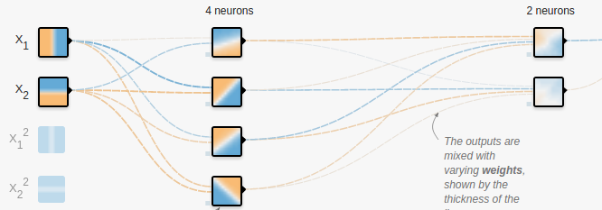
从左往右,分别是输入层,隐藏层,输出层,分别记为x,h,y.
从输入层到隐藏层的矩阵记为Whx,
偏置向量bh;
从隐藏层到输出层的矩阵记为Wyh,
偏置向量为by.
那么根据之前logistic分类的公式稍作扩展,不难得到
hz=Whxx+bhha=σ(hz)yz=Wyhha+byya=σ(yz)
其实就是两层logistic分类的堆叠,将前一个分类器的输出作为后一个的输入。得到输出ya
以后的判断方法也比较类似,哪项最高就判定属于哪一类。真正值得写一下的是神经网络中的后向算法。按照传统的logistic分类,只能做到根据误差来更新Wyh
和by
那么如何来更新从输入层到隐藏层的参数Whx和bh呢?这就要用到后向算法了。所谓后向算法,就是指误差由输出层逐层往前传递,进而逐层更新参数矩阵和偏执向量。后向算法的核心其实就4个字:链式法则。首先来看Wyh
和by的更新
C=12(ya−y)2∂C∂yz=C′σ′(yz)=(ya−y).×a.×(1−a)∂C∂Wyh=∂C∂yz∂yz∂Wyh=C′σ′(yz)hTa∂C∂by=∂C∂yz∂yz∂by=C′σ′(yz)
其实在上面的公式中,已经用到了链式法则。 类似的,可以得到
∂C∂ha=∂C∂yz∂yz∂ha=WTyh[C′σ′(yz)]∂C∂Whx=∂C∂ha∂ha∂W=[∂C∂haσ′(hz)]xT∂C∂bh=∂C∂ha∂ha∂bh=[∂C∂haσ′(hz)]
可以看到,在Whx和bh的计算中都用到了∂C∂ha
这可以看成由输出层传递到中间层的误差。那么在获得了各参数的偏导数以后,就可以对参数进行修正了
Wyh:=Wyh−η∂C∂Wyhby:=by−η∂C∂byWhx:=Whx−η∂C∂Whxbh:=bh−η∂C∂bh
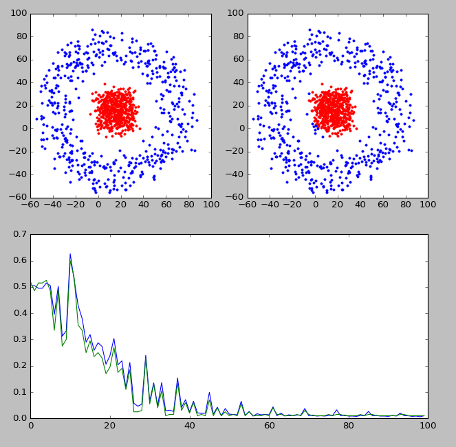
上图中,左上角显示的是实际的分类,右上角显示的是分类器判断出的各点分类。靠下的图显示的是分类器的判断准确率随迭代次数的变化情况。可以看到,经过训练以后,分类器的判断准确率还是可以的。
下面是代码部分
2
3
4
5
6
7
8
9
10
11
12
13
14
15
16
17
18
19
20
21
22
23
24
25
26
27
28
29
30
31
32
33
34
35
36
37
38
39
40
41
42
43
44
45
46
47
48
49
50
51
52
53
54
55
56
57
58
59
60
61
62
63
64
65
66
67
68
69
70
71
72
73
74
75
76
77
78
79
80
81
82
83
84
85
86
87
88
89
90
91
92
93
94
95
96
97
98
99
100
101
102
103
104
105
106
107
108
109
110
111
112
113
114
115
116
117
118
119
120
121
122
123
124
125
126
127
128
129
130
131
132
133
134
135
136
137
138
139
140
141
142
143
144

1
2
3
4
5
6
7
8
9
10
11
12
13
14
15
16
17
18
19
20
21
22
23
24
25
26
27
28
29
30
31
32
33
34
35
36
37
38
39
40
41
42
43
44
45
46
47
48
49
50
51
52
53
54
55
56
57
58
59
60
61
62
63
64
65
66
67
68
69
70
71
72
73
74
75
76
77
78
79
80
81
82
83
84
85
86
87
88
89
90
91
92
93
94
95
96
97
98
99
100
101
102
103
104
105
106
107
108
109
110
111
112
113
114
115
116
117
118
119
120
121
122
123
124
125
126
127
128
129
130
131
132
133
134
135
136
137
138
139
140
141
142
143
144
2.简单神经网络及后向传播算法
2.1 大概描述和公式表达
神经网络的大概结构如图所示,从左往右,分别是输入层,隐藏层,输出层,分别记为x,h,y.
从输入层到隐藏层的矩阵记为Whx,
偏置向量bh;
从隐藏层到输出层的矩阵记为Wyh,
偏置向量为by.
那么根据之前logistic分类的公式稍作扩展,不难得到
hz=Whxx+bhha=σ(hz)yz=Wyhha+byya=σ(yz)
其实就是两层logistic分类的堆叠,将前一个分类器的输出作为后一个的输入。得到输出ya
以后的判断方法也比较类似,哪项最高就判定属于哪一类。真正值得写一下的是神经网络中的后向算法。按照传统的logistic分类,只能做到根据误差来更新Wyh
和by
那么如何来更新从输入层到隐藏层的参数Whx和bh呢?这就要用到后向算法了。所谓后向算法,就是指误差由输出层逐层往前传递,进而逐层更新参数矩阵和偏执向量。后向算法的核心其实就4个字:链式法则。首先来看Wyh
和by的更新
C=12(ya−y)2∂C∂yz=C′σ′(yz)=(ya−y).×a.×(1−a)∂C∂Wyh=∂C∂yz∂yz∂Wyh=C′σ′(yz)hTa∂C∂by=∂C∂yz∂yz∂by=C′σ′(yz)
其实在上面的公式中,已经用到了链式法则。 类似的,可以得到
∂C∂ha=∂C∂yz∂yz∂ha=WTyh[C′σ′(yz)]∂C∂Whx=∂C∂ha∂ha∂W=[∂C∂haσ′(hz)]xT∂C∂bh=∂C∂ha∂ha∂bh=[∂C∂haσ′(hz)]
可以看到,在Whx和bh的计算中都用到了∂C∂ha
这可以看成由输出层传递到中间层的误差。那么在获得了各参数的偏导数以后,就可以对参数进行修正了
Wyh:=Wyh−η∂C∂Wyhby:=by−η∂C∂byWhx:=Whx−η∂C∂Whxbh:=bh−η∂C∂bh
2.2 神经网络的简单实现
为了加深印象,我自己实现了一个神经网络分类器,分类效果如下图所示上图中,左上角显示的是实际的分类,右上角显示的是分类器判断出的各点分类。靠下的图显示的是分类器的判断准确率随迭代次数的变化情况。可以看到,经过训练以后,分类器的判断准确率还是可以的。
下面是代码部分
import numpy as np
import matplotlib.pyplot as plt
import random
import math

# 构造各个分类
def gen_sample():
data = []
radius = [0,50]
for i in range(1000):  # 生成10k个点
catg = random.randint(0,1)  # 决定分类
r = random.random()*10
arg = random.random()*360
len = r + radius[catg]
x_c = math.cos(math.radians(arg))*len
y_c = math.sin(math.radians(arg))*len
x = random.random()*30 + x_c
y = random.random()*30 + y_c
data.append((x,y,catg))
return data

def plot_dots(data):
data_asclass = [[] for i in range(2)]
for d in data:
data_asclass[int(d[2])].append((d[0],d[1]))
colors = ['r.','b.','r.','b.']
for i,d in enumerate(data_asclass):
# print(d)
nd = np.array(d)
plt.plot(nd[:,0],nd[:,1],colors[i])
plt.draw()

def train(input, output, Whx, Wyh, bh, by):
"""
完成神经网络的训练过程
:param input:   输入列向量, 例如 [x,y].T
:param output:  输出列向量, 例如[0,1,0,0].T
:param Whx:     x->h 的参数矩阵
:param Wyh:     h->y 的参数矩阵
:param bh:      x->h 的偏置向量
:param by:      h->y 的偏置向量
:return:
"""
h_z = np.dot(Whx, input) + bh   # 线性求和
h_a = 1/(1+np.exp(-1*h_z))      # 经过sigmoid激活函数
y_z = np.dot(Wyh, h_a) + by
y_a = 1/(1+np.exp(-1*y_z))
c_y = (y_a-output)*y_a*(1-y_a)
dWyh = np.dot(c_y, h_a.T)
dby = c_y
c_h = np.dot(Wyh.T, c_y)*h_a*(1-h_a)
dWhx = np.dot(c_h,input.T)
dbh = c_h
return dWhx,dWyh,dbh,dby,c_y

def test(train_set, test_set, Whx, Wyh, bh, by):
train_tag = [int(x) for x in train_set[:,2]]
test_tag = [int(x) for x in test_set[:,2]]
train_pred = []
test_pred = []

for i,d in enumerate(train_set):
input = train_set[i:i+1,0:2].T
tag = predict(input,Whx,Wyh,bh,by)
train_pred.append(tag)
for i,d in enumerate(test_set):
input = test_set[i:i+1,0:2].T
tag = predict(input,Whx,Wyh,bh,by)
test_pred.append(tag)
# print(train_tag)
# print(train_pred)
train_err = 0
test_err = 0
for i in range(train_pred.__len__()):
if train_pred[i]!=int(train_tag[i]):
train_err += 1
for i in range(test_pred.__len__()):
if test_pred[i]!=int(test_tag[i]):
test_err += 1
# print(test_tag)
# print(test_pred)
train_ratio = train_err / train_pred.__len__()
test_ratio = test_err / test_pred.__len__()
return train_err,train_ratio,test_err,test_ratio

def predict(input,Whx,Wyh,bh,by):
# print('-----------------')
# print(input)
h_z = np.dot(Whx, input) + bh   # 线性求和
h_a = 1/(1+np.exp(-1*h_z))      # 经过sigmoid激活函数
y_z = np.dot(Wyh, h_a) + by
y_a = 1/(1+np.exp(-1*y_z))
# print(y_a)
tag = np.argmax(y_a)
return tag

if __name__=='__main__':
input_dim   = 2
output_dim  = 2
hidden_size = 200
Whx = np.random.randn(hidden_size, input_dim)*0.01
Wyh = np.random.randn(output_dim, hidden_size)*0.01
bh  = np.zeros((hidden_size, 1))
by  = np.zeros((output_dim, 1))
data = gen_sample()
plt.subplot(221)
plot_dots(data)
ndata = np.array(data)
train_set = ndata[0:800,:]
test_set = ndata[800:1000,:]
train_ratio_list = []
test_ratio_list = []
for times in range(10000):
i = times%train_set.__len__()
input = train_set[i:i+1,0:2].T
tag = int(train_set[i,2])
output = np.zeros((2,1))
output[tag,0] = 1
dWhx,dWyh,dbh,dby,c_y = train(input,output,Whx,Wyh,bh,by)
if times%100==0:
train_err,train_ratio,test_err,test_ratio = test(train_set,test_set,Whx,Wyh,bh,by)
print('times:{t}\t train ratio:{tar}\t test ratio: {ter}'.format(tar=train_ratio,ter=test_ratio,t=times))
train_ratio_list.append(train_ratio)
test_ratio_list.append(test_ratio)

for param, dparam in zip([Whx, Wyh, bh, by],
[dWhx,dWyh,dbh,dby]):
param -= 0.01*dparam
for i,d in enumerate(ndata):
input = ndata[i:i+1,0:2].T
tag = predict(input,Whx,Wyh,bh,by)
ndata[i,2] = tag
plt.subplot(222)
plot_dots(ndata)
# plt.figure()
plt.subplot(212)
plt.plot(train_ratio_list)
plt.plot(test_ratio_list)
plt.show()12
3
4
5
6
7
8
9
10
11
12
13
14
15
16
17
18
19
20
21
22
23
24
25
26
27
28
29
30
31
32
33
34
35
36
37
38
39
40
41
42
43
44
45
46
47
48
49
50
51
52
53
54
55
56
57
58
59
60
61
62
63
64
65
66
67
68
69
70
71
72
73
74
75
76
77
78
79
80
81
82
83
84
85
86
87
88
89
90
91
92
93
94
95
96
97
98
99
100
101
102
103
104
105
106
107
108
109
110
111
112
113
114
115
116
117
118
119
120
121
122
123
124
125
126
127
128
129
130
131
132
133
134
135
136
137
138
139
140
141
142
143
144
1
2
3
4
5
6
7
8
9
10
11
12
13
14
15
16
17
18
19
20
21
22
23
24
25
26
27
28
29
30
31
32
33
34
35
36
37
38
39
40
41
42
43
44
45
46
47
48
49
50
51
52
53
54
55
56
57
58
59
60
61
62
63
64
65
66
67
68
69
70
71
72
73
74
75
76
77
78
79
80
81
82
83
84
85
86
87
88
89
90
91
92
93
94
95
96
97
98
99
100
101
102
103
104
105
106
107
108
109
110
111
112
113
114
115
116
117
118
119
120
121
122
123
124
125
126
127
128
129
130
131
132
133
134
135
136
137
138
139
140
141
142
143
144

相关文章推荐
- 深度学习笔记(二):简单神经网络,后向传播算法及实现
- 深度学习基础模型算法原理及编程实现--06.循环神经网络
- 深度学习基础模型算法原理及编程实现--04.改进神经网络的方法
- 神经网络学习(四)反向(BP)传播算法(2)-Matlab实现
- python 深度学习、python神经网络算法、python数据分析、python神经网络算法数学基础教学
- 在matlab基础上简单实现一个神经网络算法
- 深度学习算法实践3---神经网络常用操作实现
- 【深度学习】1.2:简单神经网络的python实现
- 深度学习算法实践3---神经网络常用操作实现
- 深度学习算法实践3---神经网络常用操作实现
- 深度学习基础(五):循环神经网络概念、结构及原理实现
- 深度学习基础模型算法原理及编程实现--09.自编码网络
- TensorFlow:实战Google深度学习框架(二)实现简单神经网络
- [置顶] 【深度学习】RNN循环神经网络Python简单实现
- [action] deep learning 深度学习 tensorflow 实战(2) 实现简单神经网络以及随机梯度下降算法S.G.D
- 深度学习中简单神经网络的实现
- (尤其是训练集验证集的生成)深度学习 tensorflow 实战(2) 实现简单神经网络以及随机梯度下降算法S.G.D
- DAY7: 神经网络及深度学习基础--算法的优化(deeplearning.ai)
- python实现简单神经网络算法
- 如何用70行Java代码实现深度神经网络算法