xgboost原理及并行实现
2017-04-01 16:53
369 查看
XGBoost训练: It is not easy to train all the trees at once. Instead, we use an additive strategy: fix what we have learned, and add one new tree at a time. We write the prediction value at step t as $\hat{y}^{(t)}_i$,so we have
$\hat{y}^{(0)}_i = 0$
$\hat{y}^{(1)}_i = f_1(x_i) = \hat{y}^{(0)}_i + f_1(x_i)$
$\hat{y}_i^{(t)} = \sum^t_{k=1}f_k(x_i) = \hat{y}_i^{(t-1)} + f_t(x_i)$
优化目标:

If we consider using MSE(mean square error) as our loss function, it becomes the following form.

The form of MSE is friendly, with a first order(linear) term (usually called the residual) and a quadratic term. For other losses of interest (for example, logistic loss), it is not so easy to get such a nice form. So in the general case, we take the Taylor expansion of the loss function up to the second order(损失函数在上一轮模型处泰勒二阶展开)
泰勒公式:


where the $g_i$ and $h_i$ are defined as
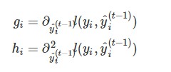
(自变量为$\hat{y}^{(t)}_i = f_t(x_i) + \hat{y}^{(t-1)}_i$,在$\hat{y}^{(t-1)}_i$处泰勒展开)
After we remove all the constants, the specific objective at step t becomes
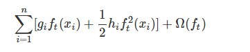
This becomes our optimization goal for the new tree. One important advantage of this definition is that it only depends on $g_i$ and $h_i$.
this is how xgboost can support custom loss functions. We can optimize every loss function, including logistic regression and weighted logistic regression, using exactly the same solver that takes $g_i$ and $h_i$ as input.
定制objective function 和evaluation function: https://github.com/dmlc/xgboost/blob/master/demo/guide-python/custom_objective.py
gbm算法:
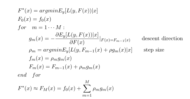
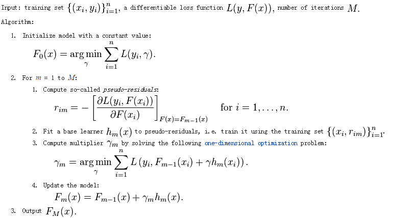
gbdt是用损失函数的负梯度在当前模型的值作为残差的近似值,拟合一个回归树,一个回归树对应着输入空间(特征空间)一个划分以及在划分的单元上的输出值。上述的gm(x)这一步有问题,应该是先利用上一步的模型计算出(近似)残差r_i,然后利用(x_i, r_i)拟合一个回归树g_m(x),以下面的伪代码为准。(参考统计学习方法8.4节)
gbdt的分类算法从思想上和gbdt的回归算法没有区别,但是由于样本输出不是连续的值,而是离散的类别,导致我们无法直接去拟合输出类别与真实类别的误差(比如说label有0和1两类,则预测类别要么0要么1,误差要么0,要么±1,而回归问题输出值是不断接近真实值)。为了解决这个问题,主要有两个方法,一个是用指数损失函数,此时GBDT退化为Adaboost算法。另一种方法是用类似于逻辑回归的对数损失函数的方法。也就是说,我们用的是类别的预测概率值和真实概率值的差来拟合损失。 参考: http://www.cnblogs.com/pinard/p/6140514.html
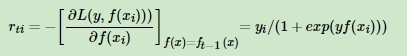
对数损失函数:

,其中

,对应的负梯度为
(我的理解:gbdt用于回归问题,使用平方损失函数;用于分类问题,使用指数损失函数,此时相当于adaboost算法中的基分类器是决策树,或使用对数损失函数,预测值是类别的概率)
使用GBDT来解决多分类问题,实质是把它转化为回归问题 。在回归问题中,GBDT每一轮迭代都构建了一棵树,实质是构建了一个函数f,当输入为x时,树的输出为f(x)。
在多分类问题中,假设有k个类别,那么每一轮迭代实质是构建了k棵树,对某个样本x的预测值为

在这里我们仿照多分类的逻辑回归,使用softmax来产生概率,则属于某个类别c的概率为 $p(y = c | x) = exp(f_c(x)) / \sum_{i = 1}^Kexp(f_i(x))$
此时该样本的loss即可以用logitloss(和softmax回归的损失函数相同)来表示,并对f1~fk都可以算出一个梯度,f1~fk便可以计算出当前轮的残差,供下一轮迭代学习,最终做预测时,输入的x会得到k个输出值,然后通过softmax获得其属于各类别的概率即可.xgboost的源码实现就是这个思路。
http://homes.cs.washington.edu/~tqchen/pdf/BoostedTree.pdf xgboost原作者ppt,看完
Model Complexity
let us first refine the definition of the tree $f(x)$ as $f_t(x) = w_{q(x)}, w \in R^T,q:R^d ->{1,2,...T} $
$w$ is the vector of scores on leaves, $q$ is a function assigning each data point to the corresponding leaf, and $T$ is the number of leaves. In XGBoost, we define the complexity as (当前树的复杂度,对于回归树,叶子节点数就是当前f函数预测值的个数,score值表示叶子节点的权重,并不是输出值,这个权重需要学习得到的 )

after reformalizing the tree model, we can write the objective value with the t-th tree as:(损失项+正则项)
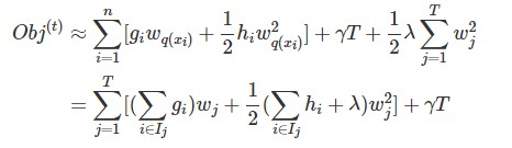
For a fixed structure q(x), we can compute the optimal weight w_j of leaf j by
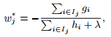
and calculate the corresponding optimal value by(当前树的损失值,作为分裂的评价标准)
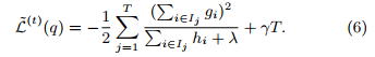
Normally it is impossible to enumerate all the possible tree structures q. A greedy algorithm that starts from a single leaf and iteratively adds branches to the tree is used instead. Assume that IL and IR are the instance sets of left and right nodes after the split. Lettting I = I_L ∪ I_R, then the loss reduction after the split is given by
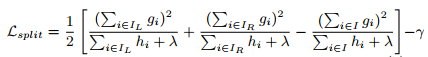
(分裂后的损失值小于父节点的损失,直接求差是个负数,所以乘以-1)
$I_j = \{i|q(x_i) = j\}$ is the set of indices of data points assigned to the j-th leaf.Notice that in the second line we have changed the index of the summation because all the data points on the same leaf get the same score.We could further compress the expression by defining $G_j = \sum_{i \in I_j}g_i$ and $H_j = \sum_{i \in I_j}h_i$:

parallel gradient boosting decision trees
gbdt is a sequential algorithm. Therefore, we can't parallelize the algorithm like Random Forest. We can only parallelize the algorithm in the tree building step. Therefore, the problem reduces to parallel decision tree building.
method 1: parallelize node building at each level(我的理解:确定好分裂特征和分裂点后,各子节点中instance已经确定,然后并行建立子节点,包括后续的节点,问题是不同节点中实例个数不平衡,workload imbalanced problem)
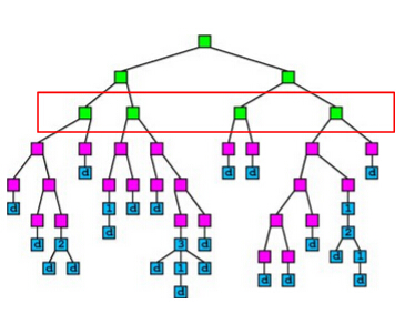
A simple idea of parallel decision tree bulding is to parallelize node building at each level. However, this method has a serious workload imbalanced problem. The reason is that a decsion tree tends to purify its nodes to obtain high prediction accuracy, and therefore many of the nodes will only contain a small group of training instances that have purified results, while some other nodes contain large group of trianing instances. The figure below shows an example of the imbalanced workload problem. Suppose we are going to build the nodes in the red box in parallel. We can see that the first and the third nodes contain much less training instances than the second and the fourth node, which causes the workload imbalanced.
method 2: parallelize split finding on each node(在每个节点中并行寻找最佳分裂特征(并行处理多个特征),如果节点中实例数目很少,并行化的好处不足以弥补多线程中上下文切换,thread join等带来的损失)
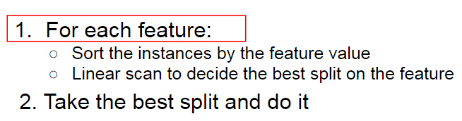
Recall that in the split finding process on a node (the process is showed below), we need to enumerate each feature to find the split. The idea of this method is to parallelize the split finding process, so that in each node, the algorithm find split for different features in parallel.
The main problem of this method is that it will has too much overhead for small nodes. When a decision tree grows deeper, most of the nodes will only contain a small number of training instances. In this case, the computation cost for each node is very small, and the benefit brought by parallel computing can not cover the overhead brought by context switching(上下文切换), thread joining, and etc., which makes the method fails to achieve a good speedup. However, this method indeed points us to a correct direction, and our final method is based on parallel split finding by features.
method 3: parallelize split finding at each level by features(对于每个特征,并行寻找在每个叶子节点上的最佳分裂点,并行处理多个特征)
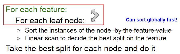
It is showed above that at each level, the sequential building process of decision tree has two loops, the first one is an outer loop for enumerating(枚举) the leaf nodes, and the second one is an inner loop that enumerates the features. The idea of this method is to swap the order of these two loops, so that we can parallelize the split finding for different features at the same level. A pseudocode of the algorithm is showed below. We can see that by changing the order of the loop, we also avoid sorting the instances in each node. We can sort the instances at the start of the whole building process, and then use the same sorting result at each level. On the other hand, note that to keep the correctness of the algorithm, each thread needs to carefully maintain their scaning status of each leaf node during the linear scan process, which significantly increases the coding complexity of the algorithm.(一个线程处理一个特征,首先在开始建树之前,将所有的数据按照该特征的特征值排序,记录排序结果。然后每一层分裂时,对于每个叶子节点中的数据逐一遍历,计算按当前数据点的特征值分裂的增益)
The advantages of the method are:
Workload are totally balanced. Since the number of instances for each feature is the same, the workload for different jobs is the same. Thus, we do not have the workload imbalanced problem in method 1.
Overhead for parallelization is small. Since we parallelize split finding at the whole level rather than a single node, the benefit from parallel computing is totally enough to cover the overhead from parallel computing
the xgboost advantage
Regularization(正则化):xgboost在损失函数中加入了正则项(见上面的公式)
Standard GBM implementation has no regularization like XGBoost, therefore it also helps to reduce overfitting.
In fact, XGBoost is also known as ‘regularized boosting‘ technique.
Parallel Processing:
XGBoost implements parallel processing and is blazingly faster as compared to GBM.
XGBoost also supports implementation on Hadoop.
High Flexibility
XGBoost allow users to define custom optimization objectives and evaluation criteria.
This adds a whole new dimension to the model and there is no limit to what we can do.
Handling Missing Values(特征值缺失的样本点分别分配到左右两个子节点中,计算增益,选择增益最大的方向作为分裂方向)
XGBoost has an in-built routine to handle missing values. <= xgboost如何处理缺失值的?
User is required to supply a different value than other observations and pass that as a parameter. XGBoost tries different things as it encounters a missing value on each node and learns which path to take for missing values in future.(缺失值指的应该是某一实例在分裂特征维度的取值不存在,这样就无法确定将它分到哪个子节点中)
Tree Pruning:
A GBM would stop splitting a node when it encounters a negative loss in the split. Thus it is more of a greedy algorithm.
XGBoost on the other hand make splits upto the max_depth specified and then start pruning the tree backwards and remove splits beyond which there is no positive gain.
Another advantage is that sometimes a split of negative loss say -2 may be followed by a split of positive loss +10. GBM would stop as it encounters -2. But XGBoost will go deeper and it will see a combined effect of +8 of the split and keep both.
Built-in Cross-Validation
XGBoost allows user to run a cross-validation at each iteration of the boosting process and thus it is easy to get the exact optimum number of boosting iterations(树的数目) in a single run.
This is unlike GBM where we have to run a grid-search and only a limited values can be tested.
Continue on Existing Model
User can start training an XGBoost model from its last iteration of previous run. This can be of significant advantage in certain specific applications.
GBM implementation of sklearn also has this feature so they are even on this point.
源码阅读以及xgboost与gbdt的区别:
http://mlnote.com/2016/10/29/xgboost-code-review-with-paper/ https://www.zhihu.com/question/41354392
1、传统GBDT在优化时只用到一阶导数信息(作为残差的近似值),xgboost则对损失函数进行了二阶泰勒展开,同时用到了一阶和二阶导数,作为损失项。顺便提一下,xgboost工具支持自定义代价函数,只要函数可一阶和二阶求导。
2、xgboost在损失函数里加入了正则项,用于控制模型的复杂度。正则项里包含了树的叶子节点个数、每个叶子节点上输出的score的L2模的平方和。从Bias-variance tradeoff角度来讲,正则项降低了模型的variance,使学习出来的模型更加简单,防止过拟合,这也是xgboost优于传统GBDT的一个特性。(L2正则 + shrinkage scales + 列采样、行采样)
3、对缺失值的处理。对于特征的值有缺失的样本,xgboost可以自动学习出它的分裂方向。
4、xgboost工具支持并行
https://arxiv.org/pdf/1603.02754.pdf xgboost原始论文
处理缺失值:
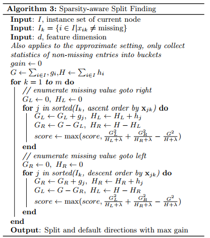
When a value is missing in the sparse matrix x, the instance is classified into the default direction. There are two choices of default direction in each branch. The optimal default directions are learnt from the data. The algorithm is shown in Alg. 3. The key improvement is to only visit the non-missing entries I_k . The presented algorithm treats the non-presence as a missing value and learns the best direction to handle missing values.
正则措施: L2正则 + shrinkage scales + 列采样、行采样
Besides the regularized objective,two additional techniques are used to further prevent over- fitting. The first technique is shrinkage introduced . Shrinkage scales newly added weights by a factor η after each step of tree boosting. Similar to a learning rate in tochastic optimization, shrinkage reduces the influence of each individual tree and leaves space for future trees to improve the model. The second technique is column (feature) subsampling. According to user feedback, using column sub-sampling prevents over-fitting even more so than the traditional row sub-sampling (which is also supported).
参考:
http://xgboost.readthedocs.io/en/latest/model.html#elements-of-supervised-learning http://zhanpengfang.github.io/418home.html https://www.analyticsvidhya.com/blog/2016/03/complete-guide-parameter-tuning-xgboost-with-codes-python/
$\hat{y}^{(0)}_i = 0$
$\hat{y}^{(1)}_i = f_1(x_i) = \hat{y}^{(0)}_i + f_1(x_i)$
$\hat{y}_i^{(t)} = \sum^t_{k=1}f_k(x_i) = \hat{y}_i^{(t-1)} + f_t(x_i)$
优化目标:
If we consider using MSE(mean square error) as our loss function, it becomes the following form.
The form of MSE is friendly, with a first order(linear) term (usually called the residual) and a quadratic term. For other losses of interest (for example, logistic loss), it is not so easy to get such a nice form. So in the general case, we take the Taylor expansion of the loss function up to the second order(损失函数在上一轮模型处泰勒二阶展开)
泰勒公式:
where the $g_i$ and $h_i$ are defined as
(自变量为$\hat{y}^{(t)}_i = f_t(x_i) + \hat{y}^{(t-1)}_i$,在$\hat{y}^{(t-1)}_i$处泰勒展开)
After we remove all the constants, the specific objective at step t becomes
This becomes our optimization goal for the new tree. One important advantage of this definition is that it only depends on $g_i$ and $h_i$.
this is how xgboost can support custom loss functions. We can optimize every loss function, including logistic regression and weighted logistic regression, using exactly the same solver that takes $g_i$ and $h_i$ as input.
定制objective function 和evaluation function: https://github.com/dmlc/xgboost/blob/master/demo/guide-python/custom_objective.py
gbm算法:
gbdt是用损失函数的负梯度在当前模型的值作为残差的近似值,拟合一个回归树,一个回归树对应着输入空间(特征空间)一个划分以及在划分的单元上的输出值。上述的gm(x)这一步有问题,应该是先利用上一步的模型计算出(近似)残差r_i,然后利用(x_i, r_i)拟合一个回归树g_m(x),以下面的伪代码为准。(参考统计学习方法8.4节)
gbdt的分类算法从思想上和gbdt的回归算法没有区别,但是由于样本输出不是连续的值,而是离散的类别,导致我们无法直接去拟合输出类别与真实类别的误差(比如说label有0和1两类,则预测类别要么0要么1,误差要么0,要么±1,而回归问题输出值是不断接近真实值)。为了解决这个问题,主要有两个方法,一个是用指数损失函数,此时GBDT退化为Adaboost算法。另一种方法是用类似于逻辑回归的对数损失函数的方法。也就是说,我们用的是类别的预测概率值和真实概率值的差来拟合损失。 参考: http://www.cnblogs.com/pinard/p/6140514.html
对数损失函数:
,其中
,对应的负梯度为
(我的理解:gbdt用于回归问题,使用平方损失函数;用于分类问题,使用指数损失函数,此时相当于adaboost算法中的基分类器是决策树,或使用对数损失函数,预测值是类别的概率)
使用GBDT来解决多分类问题,实质是把它转化为回归问题 。在回归问题中,GBDT每一轮迭代都构建了一棵树,实质是构建了一个函数f,当输入为x时,树的输出为f(x)。
在多分类问题中,假设有k个类别,那么每一轮迭代实质是构建了k棵树,对某个样本x的预测值为
在这里我们仿照多分类的逻辑回归,使用softmax来产生概率,则属于某个类别c的概率为 $p(y = c | x) = exp(f_c(x)) / \sum_{i = 1}^Kexp(f_i(x))$
此时该样本的loss即可以用logitloss(和softmax回归的损失函数相同)来表示,并对f1~fk都可以算出一个梯度,f1~fk便可以计算出当前轮的残差,供下一轮迭代学习,最终做预测时,输入的x会得到k个输出值,然后通过softmax获得其属于各类别的概率即可.xgboost的源码实现就是这个思路。
http://homes.cs.washington.edu/~tqchen/pdf/BoostedTree.pdf xgboost原作者ppt,看完
Model Complexity
let us first refine the definition of the tree $f(x)$ as $f_t(x) = w_{q(x)}, w \in R^T,q:R^d ->{1,2,...T} $
$w$ is the vector of scores on leaves, $q$ is a function assigning each data point to the corresponding leaf, and $T$ is the number of leaves. In XGBoost, we define the complexity as (当前树的复杂度,对于回归树,叶子节点数就是当前f函数预测值的个数,score值表示叶子节点的权重,并不是输出值,这个权重需要学习得到的 )
after reformalizing the tree model, we can write the objective value with the t-th tree as:(损失项+正则项)
For a fixed structure q(x), we can compute the optimal weight w_j of leaf j by
and calculate the corresponding optimal value by(当前树的损失值,作为分裂的评价标准)
Normally it is impossible to enumerate all the possible tree structures q. A greedy algorithm that starts from a single leaf and iteratively adds branches to the tree is used instead. Assume that IL and IR are the instance sets of left and right nodes after the split. Lettting I = I_L ∪ I_R, then the loss reduction after the split is given by
(分裂后的损失值小于父节点的损失,直接求差是个负数,所以乘以-1)
$I_j = \{i|q(x_i) = j\}$ is the set of indices of data points assigned to the j-th leaf.Notice that in the second line we have changed the index of the summation because all the data points on the same leaf get the same score.We could further compress the expression by defining $G_j = \sum_{i \in I_j}g_i$ and $H_j = \sum_{i \in I_j}h_i$:
https://stackoverflow.com/questions/41433209/can-someone-explain-how-these-scores-are-derived-in-this-xgboost-trees https://www.kaggle.com/general/20322
Predictions are made by summing up the corresponding leaf values of each tree. Additionally, you need to transform those values depending on the objective you have choosen. For instance: If you trained your xgb with binary:logistic, the sum of the leaf values will be the logit score. So you need to apply the logistic function to get the wanted probabilities.
Predictions are made by summing up the corresponding leaf values of each tree. Additionally, you need to transform those values depending on the objective you have choosen. For instance: If you trained your xgb with binary:logistic, the sum of the leaf values will be the logit score. So you need to apply the logistic function to get the wanted probabilities.
parallel gradient boosting decision trees
gbdt is a sequential algorithm. Therefore, we can't parallelize the algorithm like Random Forest. We can only parallelize the algorithm in the tree building step. Therefore, the problem reduces to parallel decision tree building.
method 1: parallelize node building at each level(我的理解:确定好分裂特征和分裂点后,各子节点中instance已经确定,然后并行建立子节点,包括后续的节点,问题是不同节点中实例个数不平衡,workload imbalanced problem)
A simple idea of parallel decision tree bulding is to parallelize node building at each level. However, this method has a serious workload imbalanced problem. The reason is that a decsion tree tends to purify its nodes to obtain high prediction accuracy, and therefore many of the nodes will only contain a small group of training instances that have purified results, while some other nodes contain large group of trianing instances. The figure below shows an example of the imbalanced workload problem. Suppose we are going to build the nodes in the red box in parallel. We can see that the first and the third nodes contain much less training instances than the second and the fourth node, which causes the workload imbalanced.
method 2: parallelize split finding on each node(在每个节点中并行寻找最佳分裂特征(并行处理多个特征),如果节点中实例数目很少,并行化的好处不足以弥补多线程中上下文切换,thread join等带来的损失)
Recall that in the split finding process on a node (the process is showed below), we need to enumerate each feature to find the split. The idea of this method is to parallelize the split finding process, so that in each node, the algorithm find split for different features in parallel.
The main problem of this method is that it will has too much overhead for small nodes. When a decision tree grows deeper, most of the nodes will only contain a small number of training instances. In this case, the computation cost for each node is very small, and the benefit brought by parallel computing can not cover the overhead brought by context switching(上下文切换), thread joining, and etc., which makes the method fails to achieve a good speedup. However, this method indeed points us to a correct direction, and our final method is based on parallel split finding by features.
method 3: parallelize split finding at each level by features(对于每个特征,并行寻找在每个叶子节点上的最佳分裂点,并行处理多个特征)
It is showed above that at each level, the sequential building process of decision tree has two loops, the first one is an outer loop for enumerating(枚举) the leaf nodes, and the second one is an inner loop that enumerates the features. The idea of this method is to swap the order of these two loops, so that we can parallelize the split finding for different features at the same level. A pseudocode of the algorithm is showed below. We can see that by changing the order of the loop, we also avoid sorting the instances in each node. We can sort the instances at the start of the whole building process, and then use the same sorting result at each level. On the other hand, note that to keep the correctness of the algorithm, each thread needs to carefully maintain their scaning status of each leaf node during the linear scan process, which significantly increases the coding complexity of the algorithm.(一个线程处理一个特征,首先在开始建树之前,将所有的数据按照该特征的特征值排序,记录排序结果。然后每一层分裂时,对于每个叶子节点中的数据逐一遍历,计算按当前数据点的特征值分裂的增益)
The advantages of the method are:
Workload are totally balanced. Since the number of instances for each feature is the same, the workload for different jobs is the same. Thus, we do not have the workload imbalanced problem in method 1.
Overhead for parallelization is small. Since we parallelize split finding at the whole level rather than a single node, the benefit from parallel computing is totally enough to cover the overhead from parallel computing
the xgboost advantage
Regularization(正则化):xgboost在损失函数中加入了正则项(见上面的公式)
Standard GBM implementation has no regularization like XGBoost, therefore it also helps to reduce overfitting.
In fact, XGBoost is also known as ‘regularized boosting‘ technique.
Parallel Processing:
XGBoost implements parallel processing and is blazingly faster as compared to GBM.
XGBoost also supports implementation on Hadoop.
High Flexibility
XGBoost allow users to define custom optimization objectives and evaluation criteria.
This adds a whole new dimension to the model and there is no limit to what we can do.
Handling Missing Values(特征值缺失的样本点分别分配到左右两个子节点中,计算增益,选择增益最大的方向作为分裂方向)
XGBoost has an in-built routine to handle missing values. <= xgboost如何处理缺失值的?
User is required to supply a different value than other observations and pass that as a parameter. XGBoost tries different things as it encounters a missing value on each node and learns which path to take for missing values in future.(缺失值指的应该是某一实例在分裂特征维度的取值不存在,这样就无法确定将它分到哪个子节点中)
Tree Pruning:
A GBM would stop splitting a node when it encounters a negative loss in the split. Thus it is more of a greedy algorithm.
XGBoost on the other hand make splits upto the max_depth specified and then start pruning the tree backwards and remove splits beyond which there is no positive gain.
Another advantage is that sometimes a split of negative loss say -2 may be followed by a split of positive loss +10. GBM would stop as it encounters -2. But XGBoost will go deeper and it will see a combined effect of +8 of the split and keep both.
Built-in Cross-Validation
XGBoost allows user to run a cross-validation at each iteration of the boosting process and thus it is easy to get the exact optimum number of boosting iterations(树的数目) in a single run.
This is unlike GBM where we have to run a grid-search and only a limited values can be tested.
Continue on Existing Model
User can start training an XGBoost model from its last iteration of previous run. This can be of significant advantage in certain specific applications.
GBM implementation of sklearn also has this feature so they are even on this point.
源码阅读以及xgboost与gbdt的区别:
http://mlnote.com/2016/10/29/xgboost-code-review-with-paper/ https://www.zhihu.com/question/41354392
1、传统GBDT在优化时只用到一阶导数信息(作为残差的近似值),xgboost则对损失函数进行了二阶泰勒展开,同时用到了一阶和二阶导数,作为损失项。顺便提一下,xgboost工具支持自定义代价函数,只要函数可一阶和二阶求导。
2、xgboost在损失函数里加入了正则项,用于控制模型的复杂度。正则项里包含了树的叶子节点个数、每个叶子节点上输出的score的L2模的平方和。从Bias-variance tradeoff角度来讲,正则项降低了模型的variance,使学习出来的模型更加简单,防止过拟合,这也是xgboost优于传统GBDT的一个特性。(L2正则 + shrinkage scales + 列采样、行采样)
3、对缺失值的处理。对于特征的值有缺失的样本,xgboost可以自动学习出它的分裂方向。
4、xgboost工具支持并行
https://arxiv.org/pdf/1603.02754.pdf xgboost原始论文
处理缺失值:
When a value is missing in the sparse matrix x, the instance is classified into the default direction. There are two choices of default direction in each branch. The optimal default directions are learnt from the data. The algorithm is shown in Alg. 3. The key improvement is to only visit the non-missing entries I_k . The presented algorithm treats the non-presence as a missing value and learns the best direction to handle missing values.
正则措施: L2正则 + shrinkage scales + 列采样、行采样
Besides the regularized objective,two additional techniques are used to further prevent over- fitting. The first technique is shrinkage introduced . Shrinkage scales newly added weights by a factor η after each step of tree boosting. Similar to a learning rate in tochastic optimization, shrinkage reduces the influence of each individual tree and leaves space for future trees to improve the model. The second technique is column (feature) subsampling. According to user feedback, using column sub-sampling prevents over-fitting even more so than the traditional row sub-sampling (which is also supported).
参考:
http://xgboost.readthedocs.io/en/latest/model.html#elements-of-supervised-learning http://zhanpengfang.github.io/418home.html https://www.analyticsvidhya.com/blog/2016/03/complete-guide-parameter-tuning-xgboost-with-codes-python/

相关文章推荐
- GBDT原理及实现(XGBoost+LightGBM)
- boost 库 enable_shared_from_this 实现原理分析
- 基于boost 线程并行技术实现消息队列方式[记录]
- chapter7 机器学习之元算法(adaboost)提高分类性能从原理到实现
- MySQL 5.7 并行复制实现原理与调优
- AdaBoost--从原理到实现
- boost 库 enable_shared_from_this 实现原理分析
- AdaBoost从原理到实现
- boost::bind和占位符实现的原理(from AV BOOST)
- boost::any类型实现原理
- MySQL 5.7 并行复制实现原理与调优
- boost 库 enable_shared_from_this 实现原理分析
- Boost 库 Enable_shared_from_this 实现原理分析
- boost 库 enable_shared_from_this 实现原理分析
- boost 库 enable_shared_from_this 实现原理分析
- boost::bind实现原理学习
- boost 库 enable_shared_from_this 实现原理分析
- AdaBoost--从原理到实现
- boost 库 enable_shared_from_this 实现原理分析
- AdaBoost--从原理到实现