UFLDL Exercise:Sparse Autoencoder
2016-11-26 17:51
344 查看
这是无监督特征学习和深度学习(UFLDL)的作业题。
最近入门深度学习,也没有什么matlab经验...
原网站:Exercise:Sparse Autodecoder
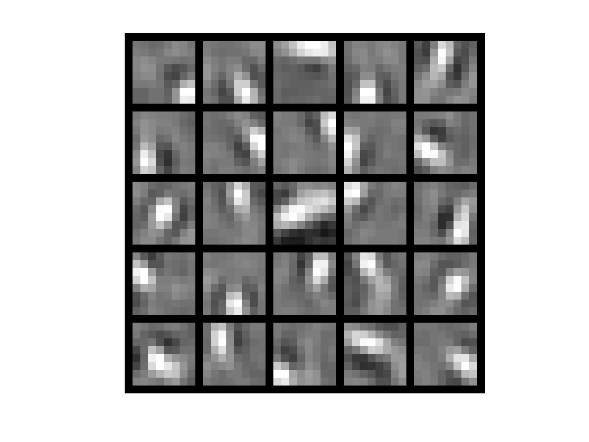
最后的J是6.5393e-11,minFunc迭代了400次,隐层能学习到的最大响应是这个样子:
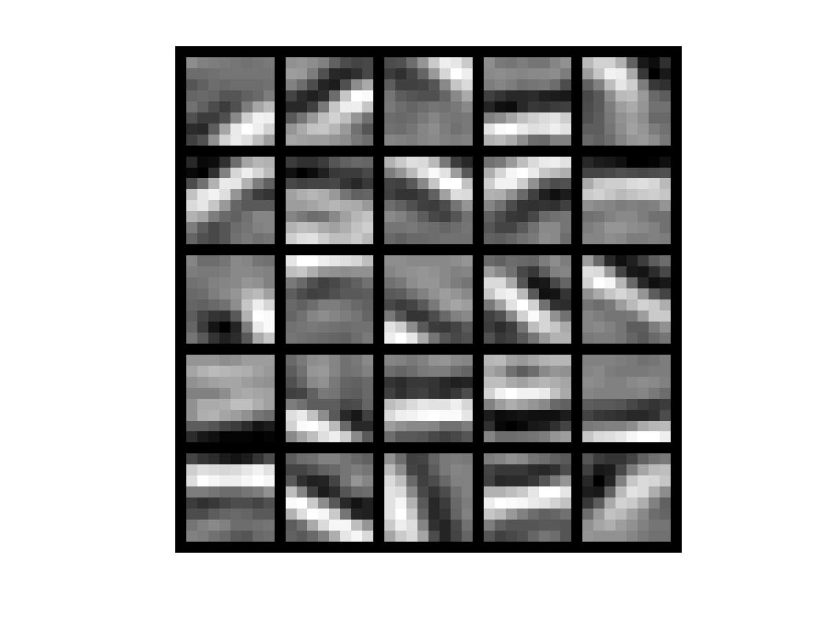
如果取消掉sparseAutodecoderCost.m中对权值更新的注释,那最终的J是0.0017,minFunc迭代了400次。隐层能学习到的最大响应是这个样子:
虽然J有所增大,但是效果明显变好。为啥权值更新了J还增大了?百思不得姐。
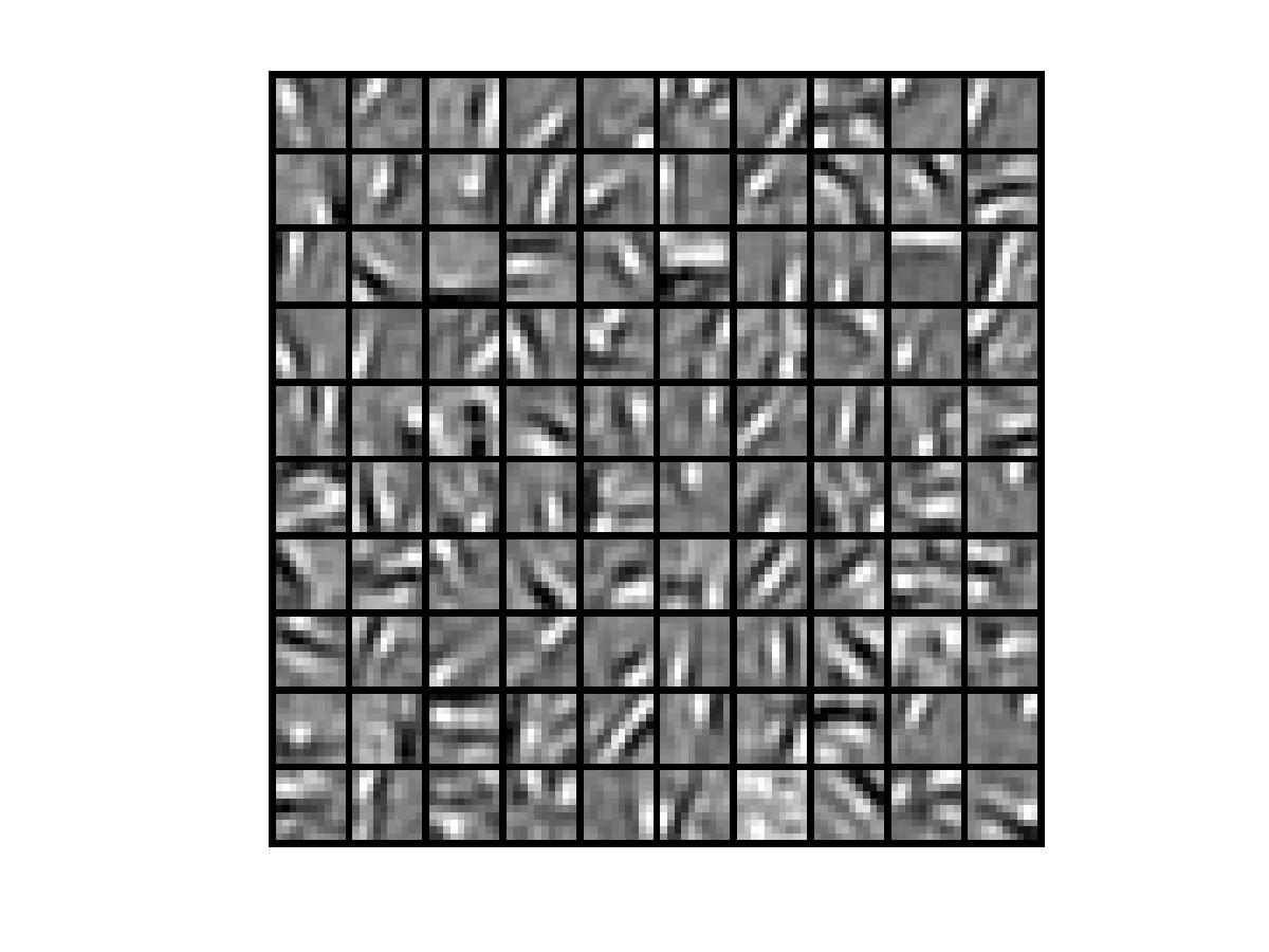
使用10*10的patch size,隐层单元为100时,J=0.0027,minFunc迭代了400次。隐层能学习到的最大响应是这个样子:
2.http://deeplearning.stanford.edu/wiki/index.php/自编码算法与稀疏性
3.http://www.cnblogs.com/tornadomeet/archive/2013/03/20/2970724.html#!comments【参照此博客修正了几个BUG】
最近入门深度学习,也没有什么matlab经验...
原网站:Exercise:Sparse Autodecoder
sampleIMAGES.m
function patches = sampleIMAGES(patchsize)
% sampleIMAGES
% Returns 10000 patches for training

load IMAGES;    % load images from disk

%patchsize = 8;  % we'll use 8x8 patches
numpatches = 10000;

% Initialize patches with zeros.  Your code will fill in this matrix--one
% column per patch, 10000 columns.
patches = zeros(patchsize*patchsize, numpatches);

%% ---------- YOUR CODE HERE --------------------------------------
%  Instructions: Fill in the variable called "patches" using data
%  from IMAGES.
%
%  IMAGES is a 3D array containing 10 images
%  For instance, IMAGES(:,:,6) is a 512x512 array containing the 6th image,
%  and you can type "imagesc(IMAGES(:,:,6)), colormap gray;" to visualize
%  it. (The contrast on these images look a bit off because they have
%  been preprocessed using using "whitening."  See the lecture notes for
%  more details.) As a second example, IMAGES(21:30,21:30,1) is an image
%  patch corresponding to the pixels in the block (21,21) to (30,30) of
%  Image 1

im_idx = randi(10);
im = IMAGES(:,:,im_idx);
parfor i = 1 : 10000
row_idx = randi(512-patchsize+1);
col_idx = randi(512-patchsize+1);
patch = im(row_idx:row_idx+patchsize-1, col_idx:col_idx+patchsize-1);
patch = reshape(patch, patchsize*patchsize, 1);
patches(:,i) = patch;
end

%% ---------------------------------------------------------------
% For the autoencoder to work well we need to normalize the data
% Specifically, since the output of the network is bounded between [0,1]
% (due to the sigmoid activation function), we have to make sure
% the range of pixel values is also bounded between [0,1]
patches = normalizeData(patches);

end

%% ---------------------------------------------------------------
function patches = normalizeData(patches)

% Squash data to [0.1, 0.9] since we use sigmoid as the activation
% function in the output layer

% Remove DC (mean of images).
patches = bsxfun(@minus, patches, mean(patches));

% Truncate to +/-3 standard deviations and scale to -1 to 1
% filter the data which is out range of [-3*sigma,3*sigma]
pstd = 3 * std(patches(:));
patches = max(min(patches, pstd), -pstd) / pstd;

% Rescale from [-1,1] to [0.1,0.9]
patches = (patches + 1) * 0.4 + 0.1;

end
sparseAutodecoderCost.m
function [cost,grad] = sparseAutoencoderCost(theta, visibleSize, hiddenSize, ...
lambda, sparsityParam, beta, data)

% visibleSize: the number of input units (probably 64)
% hiddenSize: the number of hidden units (probably 25)
% lambda: weight decay parameter
% sparsityParam: The desired average activation for the hidden units (denoted in the lecture
%                           notes by the greek alphabet rho, which looks like a lower-case "p").
% beta: weight of sparsity penalty term
% data: Our 64x10000 matrix containing the training data.  So, data(:,i) is the i-th training example.

% The input theta is a vector (because minFunc expects the parameters to be a vector).
% We first convert theta to the (W1, W2, b1, b2) matrix/vector format, so that this
% follows the notation convention of the lecture notes.
% Set the initial value of W1,W2,b1,b2 to be a zero-neighboring matrix
W1 = reshape(theta(1:hiddenSize*visibleSize), hiddenSize, visibleSize);
W2 = reshape(theta(hiddenSize*visibleSize+1:2*hiddenSize*visibleSize), visibleSize, hiddenSize);
b1 = theta(2*hiddenSize*visibleSize+1:2*hiddenSize*visibleSize+hiddenSize);
b2 = theta(2*hiddenSize*visibleSize+hiddenSize+1:end);

% Cost and gradient variables (your code needs to compute these values).
% Here, we initialize them to zeros.
W1grad = zeros(size(W1));
W2grad = zeros(size(W2));
b1grad = zeros(size(b1));
b2grad = zeros(size(b2));

%% ---------- YOUR CODE HERE --------------------------------------
%  Instructions: Compute the cost/optimization objective J_sparse(W,b) for the Sparse Autoencoder,
%                and the corresponding gradients W1grad, W2grad, b1grad, b2grad.
%
% W1grad, W2grad, b1grad and b2grad should be computed using backpropagation.
% Note that W1grad has the same dimensions as W1, b1grad has the same dimensions
% as b1, etc.  Your code should set W1grad to be the partial derivative of J_sparse(W,b) with
% respect to W1.  I.e., W1grad(i,j) should be the partial derivative of J_sparse(W,b)
% with respect to the input parameter W1(i,j).  Thus, W1grad should be equal to the term
% [(1/m) \Delta W^{(1)} + \lambda W^{(1)}] in the last block of pseudo-code in Section 2.2
% of the lecture notes (and similarly for W2grad, b1grad, b2grad).
%
% Stated differently, if we were using batch gradient descent to optimize the parameters,
% the gradient descent update to W1 would be W1 := W1 - alpha * W1grad, and similarly for W2, b1, b2.
%

n_data = size(data,2);

%1.foreward propagate to get activations
hidden_activations = sigmoid(W1 * data + repmat(b1,1,n_data));
out_activations = sigmoid(W2 * hidden_activations + repmat(b2,1,n_data));
%2.backward propagate to get residual
out_residual = -(data-out_activations).*(out_activations.*(1-out_activations));
avg_activations = sum(hidden_activations,2) ./ n_data;
KL = beta*(-sparsityParam./avg_activations + (1-sparsityParam)./(1-avg_activations));
KL = repmat(KL,1,n_data);
hidden_residual = (W2'*out_residual+KL).*(hidden_activations.*(1-hidden_activations));
%3.partial derivative and update daltaW deltab
W2grad = W2grad + out_residual * hidden_activations';
b2grad = b2grad + sum(out_residual,2);
W1grad = W1grad + hidden_residual * data';
b1grad = b1grad + sum(hidden_residual,2);

W1grad = W1grad/n_data + lambda*W1;
W2grad = W2grad/n_data + lambda*W2;
b1grad = b1grad/n_data;
b2grad = b2grad/n_data;
%4.update W1,W1,b1,b2
% alpha = 0.01;
% W1 = W1 - alpha * W1grad;
% W2 = W2 - alpha * W2grad;
% b1 = b1 - alpha * b1grad;
% b2 = b2 - alpha * b2grad;
%5.calculate cost
cost = sigmoid(W2 * sigmoid(W1 * data + repmat(b1,1,n_data)) + repmat(b2,1,n_data)) - data;
cost = sum(sum(cost.^2))/2/n_data + (lambda/2)*(sum(sum(W1.^2)) + sum(sum(W2.^2))) + ...
beta*sum(sparsityParam .* log(sparsityParam./avg_activations(:,1)) + ...
(1-sparsityParam) .* log((1-sparsityParam)./(1-avg_activations(:,1))));

%-------------------------------------------------------------------
% After computing the cost and gradient, we will convert the gradients back
% to a vector format (suitable for minFunc).  Specifically, we will unroll
% your gradient matrices into a vector.

grad = [W1grad(:) ; W2grad(:) ; b1grad(:) ; b2grad(:)];

end

%-------------------------------------------------------------------
% Here's an implementation of the sigmoid function, which you may find useful
% in your computation of the costs and the gradients.  This inputs a (row or
% column) vector (say (z1, z2, z3)) and returns (f(z1), f(z2), f(z3)).

function sigm = sigmoid(x)

sigm = 1 ./ (1 + exp(-x));
end
computeNumericalGradient.m
function numgrad = computeNumericalGradient(J, theta)
% numgrad = computeNumericalGradient(J, theta)
% theta: a vector of parameters
% J: a function that outputs a real-number. Calling y = J(theta) will return the
% function value at theta.

% Initialize numgrad with zeros
numgrad = zeros(size(theta));

%% ---------- YOUR CODE HERE --------------------------------------
% Instructions:
% Implement numerical gradient checking, and return the result in numgrad.
% (See Section 2.3 of the lecture notes.)
% You should write code so that numgrad(i) is (the numerical approximation to) the
% partial derivative of J with respect to the i-th input argument, evaluated at theta.
% I.e., numgrad(i) should be the (approximately) the partial derivative of J with
% respect to theta(i).
%
% Hint: You will probably want to compute the elements of numgrad one at a time.
EPSILON = 1e-4;
E = eye(size(theta,1));
parfor i = 1 : size(theta,1)
epsilon = E(:,i) * EPSILON;
numgrad(i) = (J(theta+epsilon) - J(theta-epsilon))/(2*EPSILON);
end
%% ---------------------------------------------------------------
end
最后的J是6.5393e-11,minFunc迭代了400次,隐层能学习到的最大响应是这个样子:
如果取消掉sparseAutodecoderCost.m中对权值更新的注释,那最终的J是0.0017,minFunc迭代了400次。隐层能学习到的最大响应是这个样子:
虽然J有所增大,但是效果明显变好。为啥权值更新了J还增大了?百思不得姐。
使用10*10的patch size,隐层单元为100时,J=0.0027,minFunc迭代了400次。隐层能学习到的最大响应是这个样子:
参考资料:
1.http://deeplearning.stanford.edu/wiki/index.php/反向传导算法2.http://deeplearning.stanford.edu/wiki/index.php/自编码算法与稀疏性
3.http://www.cnblogs.com/tornadomeet/archive/2013/03/20/2970724.html#!comments【参照此博客修正了几个BUG】

相关文章推荐
- 【UFLDL-exercise1-Sparse Autoencoder】
- UFLDL教程Exercise答案(1):Sparse Autoencoder
- UFLDL教程 Exercise:Sparse Autoencoder(答案)
- UFLDL——Exercise: Sparse Autoencoder 稀疏自动编码
- UFLDL教程: Exercise: Sparse Autoencoder
- 【UFLDL】Ex1-SparseAutoencoder 稀疏自编码器
- Convolutional neural networks(CNN) (二) Sparse Autoencoder Exercise
- UFLDL教程答案(7):Exercise:Learning color features with Sparse Autoencoders
- UFLDL(1)Sparse Autoencoder
- UFLDL教程之一 (Sparse Autoencoder练习)
- UFLDL教程: Exercise:Learning color features with Sparse Autoencoders
- 稀疏自编码http://deeplearning.stanford.edu/wiki/index.php/Exercise:Sparse_Autoencoder#Results
- Stanford UFLDL教程 Exercise:Sparse Autoencoder
- UFLDL 学习笔记——稀疏自动编码机(sparse autoencoder)
- UFLDL教程Exercise答案(7):Learning color features with Sparse Autoencoders
- UFLDL实验报告2:Sparse Autoencoder
- Convolutional neural networks(CNN) (三) Sparse Autoencoder Exercise(Vectorization)
- Exercise:Sparse Autoencoder 代码示例
- Sparse Autoencoder Exercise
- Deep Learning 1_深度学习UFLDL教程:Sparse Autoencoder练习(斯坦福大学深度学习教程)