[EverString收录]机器学习中分类评估方法简介 - 1
2016-05-13 01:49
363 查看
转自:http://blog.csdn.net/xiongtao00/article/details/51333197
----------
Classification is a kind of supervised learning, which leverages label data (ground truth) to guide the model training. Different from regression, the label here is categorical
(qualitative) rather than numeric (quantitative).
The most general classification is multi-label classification. It means there are multiple classes in the ground truth (class means label’s value) and one data point (i.e. observation or record) can belong to more than one class.
More specific, if we restrain that one data point belongs to only one class, it becomes multi-class classification or multinomial classification. In the most practical cases, we encounter multi-class classification.
Moreover, if we restrain that there are only two classes in the ground truth, then it becomes binary classification, which is the most common case.
The above definitions can be summarized by the following table:
Binary classification is simple and popular, since we usually encounter detection problems that determine whether a signal exists or not, e.g. in face detection, whether a face exists in an image, or in lead generation,
whether a company is qualified as a lead. Therefore, we start our introduction from binary classification.
In binary classification, given a data point x with
its label y (y∈{0,1}),
the classifier scores the data point as f (we
assume f∈[0,1]).
By comparing to a threshold t,
we can get the predicted label ŷ .
If f≥t,
then ŷ =1 (positive),
otherwise, ŷ =0 (negative).
For a set of N data
points X with
labels y,
the corresponding predicted scores and labels are f and ŷ ,
respectively.
Here we illustrate 3 example values that we try to predict i.e. y1, y2, y3,
we assume that we have 10 data points i=[0...9] having
scores fi in
descending order with index i.
To get ŷ ,
we use 0.5 as threshold.
From the data above, we can see that fi predicts y1,i the
best because fi value
is above 0.5 when y1,i=1;
however, fi predicts y3,i poorly.
Based on labels, the data points can be divided into positive and negative. Based on predicted labels, the data points can be divided into predicted positive and negative. We make the following basic definitions:
P:
the number of positive points, i.e. #(y=1)
N:
the number of negative points, i.e. #(y=0)
P̂ :
the number of predicted positive points, i.e. #(ŷ =1)
N̂ :
the number of predicted negative points, i.e. #(ŷ =0)
TP:
the number of predicted positive points that are actually positive, i.e. #(y=1,ŷ =1) (aka. True
Positive, Hit)
FP:
the number of predicted positive points that are actually negative, i.e. #(y=0,ŷ =1) (aka. False
Positive, False Alarm, Type I Error)
TN:
the number of predicted negative points that are actually negative, i.e. #(y=0,ŷ =0) (aka. True
Negative, Correct Rejection)
FN:
the number of predicted negative points that are actually positive, i.e. #(y=1,ŷ =0) (aka. False
Negative, Miss, Type II Error)
The above definitions can be summarized as the following confusion matrix:
Based on TP, FP, FN, TN,
we can define the following metrics:
Recall: recall=TPP=TPTP+FN,
the percentage of positive points that are predicted as positive (aka. Hit Rate, Sensitivity, True Positive Rate, TPR)
Precision: precision=TPP̂ =TPTP+FP,
the percentage of predicted positive points that are actually positive (aka. Positive Predictive value, PPV)
False Alarm Rate: fa=FPN=FPFP+TN,
the precentage of negative points that are predicted as positive (aka. False Positive Rate, FPR)
F score: f1=2⋅precision⋅recallprecision+recall,
the harmonic mean of precision and recall. It is a special case of fβ score,
when β=1.
(aka. F1 Score)
Accuracy: accuracy=TP+TNP+N,
the percentage of correct predicted points out of all points
Matthews Correlation Coefficient: MCC=TP⋅TN−FP⋅FN(TP+FP)⋅(TP+FN)⋅(TN+FP)⋅(TN+FN)√ (aka. MCC)
Mean Consequential Error: MCE=1n∑yi≠ŷ i1=FP+FNP+N=1−accuracy
In the above 3 examples, we can calculate these metrics as follows:
The following table lists the value range of each metric
* There are different ways to define the worst case. For example, the prediction that equals to random guess can be defined as worst, since it doesn’t provide any useful information. Here we define the worst case as
the prediction is totally opposite to the ground truth.
The above metrics depend on threshold, i.e. if threshold varies, the above metrics varies accordingly. To build threshold-free measurement, we can define some metrics based on labels and predicted scores (instead of
predicted labels).
The rationale is that we can measure the overall performance when the threshold goes through its value range. Here we introduce 2 curves:
ROC Curve: recall (y-axis)
vs. fa (x-axis)
curve as threshold varies
Precision-Recall Curve: precision (y-axis)
vs. recall (x-axis)
curve as threshold varies
Then we can define the following metrics:
AUC: area under ROC (Receiver Operating Characteristic) curve
Average Precision: area under precision-recall curve
Precision-Recall Breakeven Point: precision (or recall or f1 score) when precision=recall
To describe the characteristics of these curves and metrics, let’s do some case study first.
Example 1:
Example 2:
Example 3:
The above three tables list the calculation details of the recall, precision, fa and
other metrics under different thresholds for three examples, respectively. The corresponding ROC curve and precision-recall curve are plotted as follows:
From the above figures, we can summarize the characteristics of precision recall curve:
the curve is usually not monotonous
sometimes there is no definition at recall = 0, since precision is NaN (the data point with highest score is positive)
usually, as recall increases, the precision decreases with fluctuation
the curve has an intersection with line precision=recall
in the ideal case, the area under the curve is 1
The characteristics of ROC curve can be summarized as follows:
the curve is always monotonous (flat or increase)
in the best case (positive data points have higher score than negative data points), the area under the curve is 1
in the worst case (positive data points have lower score than negative data points), the area under the curve is 0
in the random case (random scoring), the area under the curve is 0.5
The following table summarizes auc, average precision and breakeven point in these three examples
The following table lists the value range of each metric
* in the case that there is no positive sample, average precison can achieve 0.
We have introduced several metrics to measure the performance of binary classification. In a practical case, what metrics should we adopt and what metrics should be avoided?
Usually, there are two cases we can encounter: balanced and unbalanced.
In balanced case, the number of positive samples is close to that of negative samples
In unbalanced case, there are orders of magnitude difference between numbers of positive and negative samples.
In practical case, positive number is usually less than negative number
The conclusions are that
In balanced case, all the above metrics can be used
In unbalanced case, precision, recall, f1 score, average precision and breakeven point are preferred rather than fa, accuracy, MCC, MCE, auc, ATOP*
*ATOP is another metric, which is similar to AUC that also cares about the order of positive and negative data points.
The main reason is that
precision, recall, f1 score, average precision, breakeven point focus on the correctness of the positive samples (related to TP,
but not TN)
fa, accuracy, MCC, MCE, auc, ATOP are related to the correctness of the negative samples (TN)
In unbalanced case, TN is
usually huge, comparing to TP.
Therefore, fa≈0, accuracy≈1, MCC≈1, MCE≈0, auc≈1, ATOP≈1.
However, these “amazing” values don’t make any sense.
Let consider the following 4 examples:
Consider example 1 and 2. The former is balanced and the latter is unbalanced. The orders of the positive samples are the same in both examples.
However, auc and atop change a lot (0.85333 vs. 0.99779, 0.79000 vs. 0.99580). The more unbalanced the case is, auc and atop tend to be higher.
average precisions in both examples are the same (0.62508 vs. 0.62508)
Consider example 3 and 4. Both of them are extremely unbalanced. The difference is that the positive samples in example 3 are ordered from 100~199 while in example 4 ordered from 0~99.
However, auc and atop are nearly the same in both cases (0.99990 vs. 1.0, 0.99985 vs. 0.99995)
the average precision is able to distinguish this difference obviously (0.30685 vs. 1.0)
-------
作者简介:熊涛,资深数据科学家,现任EverString数据科学团队中国负责人,前Hulu数据科学主管。

----------
1. Classification problem
Classification is a kind of supervised learning, which leverages label data (ground truth) to guide the model training. Different from regression, the label here is categorical(qualitative) rather than numeric (quantitative).
The most general classification is multi-label classification. It means there are multiple classes in the ground truth (class means label’s value) and one data point (i.e. observation or record) can belong to more than one class.
More specific, if we restrain that one data point belongs to only one class, it becomes multi-class classification or multinomial classification. In the most practical cases, we encounter multi-class classification.
Moreover, if we restrain that there are only two classes in the ground truth, then it becomes binary classification, which is the most common case.
The above definitions can be summarized by the following table:
| type of classification | multiple classes (in the ground truth) | two classes (in the ground truth) |
|---|---|---|
| multiple labels (one record has) | multi-label classification | – |
| single label (one record has) | multi-class classification | binary classification |
whether a company is qualified as a lead. Therefore, we start our introduction from binary classification.
2. Metrics for binary classification
2.1. Binary classification
In binary classification, given a data point x withits label y (y∈{0,1}),
the classifier scores the data point as f (we
assume f∈[0,1]).
By comparing to a threshold t,
we can get the predicted label ŷ .
If f≥t,
then ŷ =1 (positive),
otherwise, ŷ =0 (negative).
For a set of N data
points X with
labels y,
the corresponding predicted scores and labels are f and ŷ ,
respectively.
2.2. Examples
Here we illustrate 3 example values that we try to predict i.e. y1, y2, y3,we assume that we have 10 data points i=[0...9] having
scores fi in
descending order with index i.
To get ŷ ,
we use 0.5 as threshold.
| i | 0 | 1 | 2 | 3 | 4 | 5 | 6 | 7 | 8 | 9 |
|---|---|---|---|---|---|---|---|---|---|---|
| y1,i | 1 | 1 | 1 | 1 | 1 | 0 | 0 | 0 | 0 | 0 |
| y2,i | 1 | 0 | 1 | 0 | 1 | 0 | 0 | 1 | 1 | 0 |
| y3,i | 0 | 0 | 0 | 0 | 0 | 1 | 1 | 1 | 1 | 1 |
| fi | 0.96 | 0.91 | 0.75 | 0.62 | 0.58 | 0.52 | 0.45 | 0.28 | 0.17 | 0.13 |
| ŷ i | 1 | 1 | 1 | 1 | 1 | 1 | 0 | 0 | 0 | 0 |
best because fi value
is above 0.5 when y1,i=1;
however, fi predicts y3,i poorly.
2.3. Metrics based on labels and predicted labels
Based on labels, the data points can be divided into positive and negative. Based on predicted labels, the data points can be divided into predicted positive and negative. We make the following basic definitions:P:
the number of positive points, i.e. #(y=1)
N:
the number of negative points, i.e. #(y=0)
P̂ :
the number of predicted positive points, i.e. #(ŷ =1)
N̂ :
the number of predicted negative points, i.e. #(ŷ =0)
TP:
the number of predicted positive points that are actually positive, i.e. #(y=1,ŷ =1) (aka. True
Positive, Hit)
FP:
the number of predicted positive points that are actually negative, i.e. #(y=0,ŷ =1) (aka. False
Positive, False Alarm, Type I Error)
TN:
the number of predicted negative points that are actually negative, i.e. #(y=0,ŷ =0) (aka. True
Negative, Correct Rejection)
FN:
the number of predicted negative points that are actually positive, i.e. #(y=1,ŷ =0) (aka. False
Negative, Miss, Type II Error)
The above definitions can be summarized as the following confusion matrix:
| confusion matrix | P̂ | N̂ |
|---|---|---|
| P | TP | FN |
| N | FP | TN |
we can define the following metrics:
Recall: recall=TPP=TPTP+FN,
the percentage of positive points that are predicted as positive (aka. Hit Rate, Sensitivity, True Positive Rate, TPR)
Precision: precision=TPP̂ =TPTP+FP,
the percentage of predicted positive points that are actually positive (aka. Positive Predictive value, PPV)
False Alarm Rate: fa=FPN=FPFP+TN,
the precentage of negative points that are predicted as positive (aka. False Positive Rate, FPR)
F score: f1=2⋅precision⋅recallprecision+recall,
the harmonic mean of precision and recall. It is a special case of fβ score,
when β=1.
(aka. F1 Score)
Accuracy: accuracy=TP+TNP+N,
the percentage of correct predicted points out of all points
Matthews Correlation Coefficient: MCC=TP⋅TN−FP⋅FN(TP+FP)⋅(TP+FN)⋅(TN+FP)⋅(TN+FN)√ (aka. MCC)
Mean Consequential Error: MCE=1n∑yi≠ŷ i1=FP+FNP+N=1−accuracy
In the above 3 examples, we can calculate these metrics as follows:
| Metrics | TP | FP | TN | FN | recall | precision | f1 | fa | accuracy | MCC | MCE |
|---|---|---|---|---|---|---|---|---|---|---|---|
| 1 | 5 | 1 | 4 | 0 | 1 | 0.833 | 0.909 | 0.2 | 0.9 | 0.817 | 0.1 |
| 2 | 3 | 3 | 2 | 2 | 0.6 | 0.5 | 0.545 | 0.6 | 0.5 | 0 | 0.5 |
| 3 | 1 | 5 | 0 | 4 | 0.2 | 0.167 | 0.182 | 1 | 0.1 | -0.817 | 0.9 |
| Metrics | TP | FP | TN | FN | recall | precision | f1 | fa | accuracy | MCC | MCE |
|---|---|---|---|---|---|---|---|---|---|---|---|
| Range | [0,P] | [0,N] | [0,N] | [0,P] | [0,1] | [0,1] | [0,1] | [0,1] | [0,1] | [-1,1] | [0,1] |
| Best | P | 0 | N | 0 | 1 | 1 | 1 | 0 | 1 | 1 | 0 |
| Worst* | 0 | P | 0 | N | 0 | 0 | 0 | 1 | 0 | -1 | 1 |
the prediction is totally opposite to the ground truth.
2.4. Metrics based on labels and predicted scores
The above metrics depend on threshold, i.e. if threshold varies, the above metrics varies accordingly. To build threshold-free measurement, we can define some metrics based on labels and predicted scores (instead ofpredicted labels).
The rationale is that we can measure the overall performance when the threshold goes through its value range. Here we introduce 2 curves:
ROC Curve: recall (y-axis)
vs. fa (x-axis)
curve as threshold varies
Precision-Recall Curve: precision (y-axis)
vs. recall (x-axis)
curve as threshold varies
Then we can define the following metrics:
AUC: area under ROC (Receiver Operating Characteristic) curve
Average Precision: area under precision-recall curve
Precision-Recall Breakeven Point: precision (or recall or f1 score) when precision=recall
To describe the characteristics of these curves and metrics, let’s do some case study first.
Example 1:
| index | 0 | 1 | 2 | 3 | 4 | 5 | 6 | 7 | 8 | 9 | |
|---|---|---|---|---|---|---|---|---|---|---|---|
| fi | 0.96 | 0.91 | 0.75 | 0.62 | 0.58 | 0.52 | 0.45 | 0.28 | 0.17 | 0.13 | |
| y1,i | 1 | 1 | 1 | 1 | 1 | 0 | 0 | 0 | 0 | 0 | |
| threshold range | (0.96, 1] | (0.91, 0.96] | (0.75, 0.91] | (0.62, 0.75] | (0.58, 0.62] | (0.52, 0.58] | (0.45, 0.52] | (0.28, 0.45] | (0.17, 0.28] | (0.13, 0.17] | [0, 0.13] |
| TP | 0 | 1 | 2 | 3 | 4 | 5 | 5 | 5 | 5 | 5 | 5 |
| FP | 0 | 0 | 0 | 0 | 0 | 0 | 1 | 2 | 3 | 4 | 5 |
| TN | 5 | 5 | 5 | 5 | 5 | 5 | 4 | 3 | 2 | 1 | 0 |
| FN | 5 | 4 | 3 | 2 | 1 | 0 | 0 | 0 | 0 | 0 | 0 |
| recall | 0 | 0.2 | 0.4 | 0.6 | 0.8 | 1 | 1 | 1 | 1 | 1 | 1 |
| precision | NaN | 1 | 1 | 1 | 1 | 1 | 0.833 | 0.714 | 0.625 | 0.556 | 0.5 |
| f1 | NaN | 0.333 | 0.571 | 0.75 | 0.889 | 1 | 0.909 | 0.833 | 0.769 | 0.714 | 0.667 |
| fa | 0 | 0 | 0 | 0 | 0 | 0 | 0.2 | 0.4 | 0.6 | 0.8 | 1 |
| accuracy | 0.5 | 0.6 | 0.7 | 0.8 | 0.9 | 1 | 0.9 | 0.8 | 0.7 | 0.6 | 0.5 |
| MCC | NaN | 0.333 | 0.5 | 0.655 | 0.816 | 1 | 0.816 | 0.655 | 0.5 | 0.333 | NaN |
| MCE | 0.5 | 0.4 | 0.3 | 0.2 | 0.1 | 0 | 0.1 | 0.2 | 0.3 | 0.4 | 0.5 |
| index | 0 | 1 | 2 | 3 | 4 | 5 | 6 | 7 | 8 | 9 | |
|---|---|---|---|---|---|---|---|---|---|---|---|
| fi | 0.96 | 0.91 | 0.75 | 0.62 | 0.58 | 0.52 | 0.45 | 0.28 | 0.17 | 0.13 | |
| y2,i | 1 | 1 | 1 | 1 | 1 | 0 | 0 | 0 | 0 | 0 | |
| threshold range | (0.96, 1] | (0.91, 0.96] | (0.75, 0.91] | (0.62, 0.75] | (0.58, 0.62] | (0.52, 0.58] | (0.45, 0.52] | (0.28, 0.45] | (0.17, 0.28] | (0.13, 0.17] | [0, 0.13] |
| TP | 0 | 1 | 1 | 2 | 2 | 3 | 3 | 3 | 4 | 5 | 5 |
| FP | 0 | 0 | 1 | 1 | 2 | 2 | 3 | 4 | 4 | 4 | 5 |
| TN | 5 | 5 | 4 | 4 | 3 | 3 | 2 | 1 | 1 | 1 | 0 |
| FN | 5 | 4 | 4 | 3 | 3 | 2 | 2 | 2 | 1 | 0 | 0 |
| recall | 0 | 0.2 | 0.2 | 0.4 | 0.4 | 0.6 | 0.6 | 0.6 | 0.8 | 1 | 1 |
| precision | NaN | 1 | 0.5 | 0.667 | 0.5 | 0.6 | 0.5 | 0.429 | 0.5 | 0.556 | 0.5 |
| f1 | NaN | 0.333 | 0.286 | 0.5 | 0.444 | 0.6 | 0.545 | 0.5 | 0.615 | 0.714 | 0.667 |
| fa | 0 | 0 | 0.2 | 0.2 | 0.4 | 0.4 | 0.6 | 0.8 | 0.8 | 0.8 | 1 |
| accuracy | 0.5 | 0.6 | 0.5 | 0.6 | 0.5 | 0.6 | 0.5 | 0.4 | 0.5 | 0.6 | 0.5 |
| MCC | NaN | 0.333 | 0 | 0.218 | 0 | 0.2 | 0 | -0.218 | 0 | 0.333 | NaN |
| MCE | 0.5 | 0.4 | 0.5 | 0.4 | 0.5 | 0.4 | 0.5 | 0.6 | 0.5 | 0.4 | 0.5 |
| index | 0 | 1 | 2 | 3 | 4 | 5 | 6 | 7 | 8 | 9 | |
|---|---|---|---|---|---|---|---|---|---|---|---|
| fi | 0.96 | 0.91 | 0.75 | 0.62 | 0.58 | 0.52 | 0.45 | 0.28 | 0.17 | 0.13 | |
| y3,i | 1 | 1 | 1 | 1 | 1 | 0 | 0 | 0 | 0 | 0 | |
| threshold range | (0.96, 1] | (0.91, 0.96] | (0.75, 0.91] | (0.62, 0.75] | (0.58, 0.62] | (0.52, 0.58] | (0.45, 0.52] | (0.28, 0.45] | (0.17, 0.28] | (0.13, 0.17] | [0, 0.13] |
| TP | 0 | 0 | 0 | 0 | 0 | 0 | 1 | 2 | 3 | 4 | 5 |
| FP | 0 | 1 | 2 | 3 | 4 | 5 | 5 | 5 | 5 | 5 | 5 |
| TN | 5 | 4 | 3 | 2 | 1 | 0 | 0 | 0 | 0 | 0 | 0 |
| FN | 5 | 5 | 5 | 5 | 5 | 5 | 4 | 3 | 2 | 1 | 0 |
| recall | 0 | 0 | 0 | 0 | 0 | 0 | 0.2 | 0.4 | 0.6 | 0.8 | 1 |
| precision | NaN | 0 | 0 | 0 | 0 | 0 | 0.167 | 0.286 | 0.375 | 0.444 | 0.5 |
| f1 | NaN | NaN | NaN | NaN | NaN | NaN | 0.182 | 0.333 | 0.462 | 0.571 | 0.667 |
| fa | 0 | 0.2 | 0.4 | 0.6 | 0.8 | 1 | 1 | 1 | 1 | 1 | 1 |
| accuracy | 0.5 | 0.4 | 0.3 | 0.2 | 0.1 | 0 | 0.1 | 0.2 | 0.3 | 0.4 | 0.5 |
| MCC | NaN | -0.333 | -0.5 | -0.655 | -0.816 | -1 | -0.816 | -0.655 | -0.5 | -0.333 | NaN |
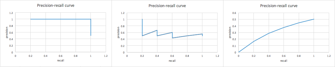
| MCE | 0.5 | 0.6 | 0.7 | 0.8 | 0.9 | 1 | 0.9 | 0.8 | 0.7 | 0.6 | 0.5 |
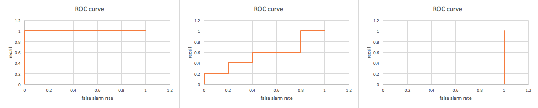
other metrics under different thresholds for three examples, respectively. The corresponding ROC curve and precision-recall curve are plotted as follows:
From the above figures, we can summarize the characteristics of precision recall curve:
the curve is usually not monotonous
sometimes there is no definition at recall = 0, since precision is NaN (the data point with highest score is positive)
usually, as recall increases, the precision decreases with fluctuation
the curve has an intersection with line precision=recall
in the ideal case, the area under the curve is 1
The characteristics of ROC curve can be summarized as follows:
the curve is always monotonous (flat or increase)
in the best case (positive data points have higher score than negative data points), the area under the curve is 1
in the worst case (positive data points have lower score than negative data points), the area under the curve is 0
in the random case (random scoring), the area under the curve is 0.5
The following table summarizes auc, average precision and breakeven point in these three examples
| metrics | auc | average precision | breakeven point |
|---|---|---|---|
| 1 | 1.000 | 1.000 | 1.000 |
| 2 | 0.565 | 0.467 | 0.600 |
| 3 | 0.000 | 0.304 | 0.000 |
| metrics | auc | average precision | breakeven point |
|---|---|---|---|
| Range | [0,1] | [0,1] | [0,1] |
| Best | 1 | 1 | 1 |
| Worst | 0 | 0* | 0 |
2.5. Metrics selection
We have introduced several metrics to measure the performance of binary classification. In a practical case, what metrics should we adopt and what metrics should be avoided?Usually, there are two cases we can encounter: balanced and unbalanced.
In balanced case, the number of positive samples is close to that of negative samples
In unbalanced case, there are orders of magnitude difference between numbers of positive and negative samples.
In practical case, positive number is usually less than negative number
The conclusions are that
In balanced case, all the above metrics can be used
In unbalanced case, precision, recall, f1 score, average precision and breakeven point are preferred rather than fa, accuracy, MCC, MCE, auc, ATOP*
*ATOP is another metric, which is similar to AUC that also cares about the order of positive and negative data points.
The main reason is that
precision, recall, f1 score, average precision, breakeven point focus on the correctness of the positive samples (related to TP,
but not TN)
fa, accuracy, MCC, MCE, auc, ATOP are related to the correctness of the negative samples (TN)
In unbalanced case, TN is
usually huge, comparing to TP.
Therefore, fa≈0, accuracy≈1, MCC≈1, MCE≈0, auc≈1, ATOP≈1.
However, these “amazing” values don’t make any sense.
Let consider the following 4 examples:
<code class="language-python hljs  has-numbering" style="display: block; padding: 0px; background-color: transparent; color: inherit; box-sizing: border-box; font-family: 'Source Code Pro', monospace;font-size:undefined; white-space: pre; border-top-left-radius: 0px; border-top-right-radius: 0px; border-bottom-right-radius: 0px; border-bottom-left-radius: 0px; word-wrap: normal; background-position: initial initial; background-repeat: initial initial;"><span class="hljs-keyword" style="color: rgb(0, 0, 136); box-sizing: border-box;">import</span> numpy <span class="hljs-keyword" style="color: rgb(0, 0, 136); box-sizing: border-box;">as</span> np
<span class="hljs-keyword" style="color: rgb(0, 0, 136); box-sizing: border-box;">from</span> sklearn.metrics <span class="hljs-keyword" style="color: rgb(0, 0, 136); box-sizing: border-box;">import</span> roc_auc_score, average_precision_score
<span class="hljs-function" style="box-sizing: border-box;"><span class="hljs-keyword" style="color: rgb(0, 0, 136); box-sizing: border-box;">def</span> <span class="hljs-title" style="box-sizing: border-box;">atop</span><span class="hljs-params" style="color: rgb(102, 0, 102); box-sizing: border-box;">(y_sorted)</span>:</span>
num = len(y_sorted)
index = range(num)
atop = <span class="hljs-number" style="color: rgb(0, 102, 102); box-sizing: border-box;">1</span> - float(sum(y_sorted * index)) / sum(y_sorted) / num
<span class="hljs-keyword" style="color: rgb(0, 0, 136); box-sizing: border-box;">return</span> atop

y1 = np.array([<span class="hljs-number" style="color: rgb(0, 102, 102); box-sizing: border-box;">1</span>,<span class="hljs-number" style="color: rgb(0, 102, 102); box-sizing: border-box;">0</span>,<span class="hljs-number" style="color: rgb(0, 102, 102); box-sizing: border-box;">1</span>,<span class="hljs-number" style="color: rgb(0, 102, 102); box-sizing: border-box;">0</span>,<span class="hljs-number" style="color: rgb(0, 102, 102); box-sizing: border-box;">1</span>,<span class="hljs-number" style="color: rgb(0, 102, 102); box-sizing: border-box;">0</span>,<span class="hljs-number" style="color: rgb(0, 102, 102); box-sizing: border-box;">0</span>,<span class="hljs-number" style="color: rgb(0, 102, 102); box-sizing: border-box;">1</span>,<span class="hljs-number" style="color: rgb(0, 102, 102); box-sizing: border-box;">1</span>,<span class="hljs-number" style="color: rgb(0, 102, 102); box-sizing: border-box;">0</span>] + [<span class="hljs-number" style="color: rgb(0, 102, 102); box-sizing: border-box;">0</span>] * <span class="hljs-number" style="color: rgb(0, 102, 102); box-sizing: border-box;">10</span>)
f1 = np.array([i / float(len(y1)) <span class="hljs-keyword" style="color: rgb(0, 0, 136); box-sizing: border-box;">for</span> i <span class="hljs-keyword" style="color: rgb(0, 0, 136); box-sizing: border-box;">in</span> range(len(y1), <span class="hljs-number" style="color: rgb(0, 102, 102); box-sizing: border-box;">0</span>, -<span class="hljs-number" style="color: rgb(0, 102, 102); box-sizing: border-box;">1</span>)])
auc1 = roc_auc_score(y1, f1)
ap1 = average_precision_score(y1, f1)
atop1 = atop(y1)
<span class="hljs-keyword" style="color: rgb(0, 0, 136); box-sizing: border-box;">print</span> auc1, atop1, ap1

y2 = np.array([<span class="hljs-number" style="color: rgb(0, 102, 102); box-sizing: border-box;">1</span>,<span class="hljs-number" style="color: rgb(0, 102, 102); box-sizing: border-box;">0</span>,<span class="hljs-number" style="color: rgb(0, 102, 102); box-sizing: border-box;">1</span>,<span class="hljs-number" style="color: rgb(0, 102, 102); box-sizing: border-box;">0</span>,<span class="hljs-number" style="color: rgb(0, 102, 102); box-sizing: border-box;">1</span>,<span class="hljs-number" style="color: rgb(0, 102, 102); box-sizing: border-box;">0</span>,<span class="hljs-number" style="color: rgb(0, 102, 102); box-sizing: border-box;">0</span>,<span class="hljs-number" style="color: rgb(0, 102, 102); box-sizing: border-box;">1</span>,<span class="hljs-number" style="color: rgb(0, 102, 102); box-sizing: border-box;">1</span>,<span class="hljs-number" style="color: rgb(0, 102, 102); box-sizing: border-box;">0</span>] + [<span class="hljs-number" style="color: rgb(0, 102, 102); box-sizing: border-box;">0</span>] * <span class="hljs-number" style="color: rgb(0, 102, 102); box-sizing: border-box;">990</span>)
f2 = np.array([i / float(len(y2)) <span class="hljs-keyword" style="color: rgb(0, 0, 136); box-sizing: border-box;">for</span> i <span class="hljs-keyword" style="color: rgb(0, 0, 136); box-sizing: border-box;">in</span> range(len(y2), <span class="hljs-number" style="color: rgb(0, 102, 102); box-sizing: border-box;">0</span>, -<span class="hljs-number" style="color: rgb(0, 102, 102); box-sizing: border-box;">1</span>)])
auc2 = roc_auc_score(y2, f2)
atop2 = atop(y2)
ap2 = average_precision_score(y2, f2)
<span class="hljs-keyword" style="color: rgb(0, 0, 136); box-sizing: border-box;">print</span> auc2, atop2, ap2

y3 = np.array([<span class="hljs-number" style="color: rgb(0, 102, 102); box-sizing: border-box;">0</span>] * <span class="hljs-number" style="color: rgb(0, 102, 102); box-sizing: border-box;">100</span> + [<span class="hljs-number" style="color: rgb(0, 102, 102); box-sizing: border-box;">1</span>] * <span class="hljs-number" style="color: rgb(0, 102, 102); box-sizing: border-box;">100</span> + [<span class="hljs-number" style="color: rgb(0, 102, 102); box-sizing: border-box;">0</span>] * <span class="hljs-number" style="color: rgb(0, 102, 102); box-sizing: border-box;">999800</span>)
f3 = np.array([i / float(len(y3)) <span class="hljs-keyword" style="color: rgb(0, 0, 136); box-sizing: border-box;">for</span> i <span class="hljs-keyword" style="color: rgb(0, 0, 136); box-sizing: border-box;">in</span> range(len(y3), <span class="hljs-number" style="color: rgb(0, 102, 102); box-sizing: border-box;">0</span>, -<span class="hljs-number" style="color: rgb(0, 102, 102); box-sizing: border-box;">1</span>)])
auc3 = roc_auc_score(y3, f3)
atop3 = atop(y3)
ap3 = average_precision_score(y3, f3)
<span class="hljs-keyword" style="color: rgb(0, 0, 136); box-sizing: border-box;">print</span> auc3, atop3, ap3

y4 = np.array([<span class="hljs-number" style="color: rgb(0, 102, 102); box-sizing: border-box;">1</span>] * <span class="hljs-number" style="color: rgb(0, 102, 102); box-sizing: border-box;">100</span> + [<span class="hljs-number" style="color: rgb(0, 102, 102); box-sizing: border-box;">0</span>] * <span class="hljs-number" style="color: rgb(0, 102, 102); box-sizing: border-box;">999900</span>)
f4 = np.array([i / float(len(y4)) <span class="hljs-keyword" style="color: rgb(0, 0, 136); box-sizing: border-box;">for</span> i <span class="hljs-keyword" style="color: rgb(0, 0, 136); box-sizing: border-box;">in</span> range(len(y4), <span class="hljs-number" style="color: rgb(0, 102, 102); box-sizing: border-box;">0</span>, -<span class="hljs-number" style="color: rgb(0, 102, 102); box-sizing: border-box;">1</span>)])
auc4 = roc_auc_score(y4, f4)
atop4 = atop(y4)
ap4 = average_precision_score(y4, f4)
<span class="hljs-keyword" style="color: rgb(0, 0, 136); box-sizing: border-box;">print</span> auc4, atop4, ap4</code><ul class="pre-numbering" style="box-sizing: border-box; position: absolute; width: 50px; background-color: rgb(238, 238, 238); top: 0px; left: 0px; margin: 0px; padding: 6px 0px 40px; border-right-width: 1px; border-right-style: solid; border-right-color: rgb(221, 221, 221); list-style: none; text-align: right;"><li style="box-sizing: border-box; padding: 0px 5px;">1</li><li style="box-sizing: border-box; padding: 0px 5px;">2</li><li style="box-sizing: border-box; padding: 0px 5px;">3</li><li style="box-sizing: border-box; padding: 0px 5px;">4</li><li style="box-sizing: border-box; padding: 0px 5px;">5</li><li style="box-sizing: border-box; padding: 0px 5px;">6</li><li style="box-sizing: border-box; padding: 0px 5px;">7</li><li style="box-sizing: border-box; padding: 0px 5px;">8</li><li style="box-sizing: border-box; padding: 0px 5px;">9</li><li style="box-sizing: border-box; padding: 0px 5px;">10</li><li style="box-sizing: border-box; padding: 0px 5px;">11</li><li style="box-sizing: border-box; padding: 0px 5px;">12</li><li style="box-sizing: border-box; padding: 0px 5px;">13</li><li style="box-sizing: border-box; padding: 0px 5px;">14</li><li style="box-sizing: border-box; padding: 0px 5px;">15</li><li style="box-sizing: border-box; padding: 0px 5px;">16</li><li style="box-sizing: border-box; padding: 0px 5px;">17</li><li style="box-sizing: border-box; padding: 0px 5px;">18</li><li style="box-sizing: border-box; padding: 0px 5px;">19</li><li style="box-sizing: border-box; padding: 0px 5px;">20</li><li style="box-sizing: border-box; padding: 0px 5px;">21</li><li style="box-sizing: border-box; padding: 0px 5px;">22</li><li style="box-sizing: border-box; padding: 0px 5px;">23</li><li style="box-sizing: border-box; padding: 0px 5px;">24</li><li style="box-sizing: border-box; padding: 0px 5px;">25</li><li style="box-sizing: border-box; padding: 0px 5px;">26</li><li style="box-sizing: border-box; padding: 0px 5px;">27</li><li style="box-sizing: border-box; padding: 0px 5px;">28</li><li style="box-sizing: border-box; padding: 0px 5px;">29</li><li style="box-sizing: border-box; padding: 0px 5px;">30</li><li style="box-sizing: border-box; padding: 0px 5px;">31</li><li style="box-sizing: border-box; padding: 0px 5px;">32</li><li style="box-sizing: border-box; padding: 0px 5px;">33</li><li style="box-sizing: border-box; padding: 0px 5px;">34</li><li style="box-sizing: border-box; padding: 0px 5px;">35</li></ul><ul class="pre-numbering" style="box-sizing: border-box; position: absolute; width: 50px; background-color: rgb(238, 238, 238); top: 0px; left: 0px; margin: 0px; padding: 6px 0px 40px; border-right-width: 1px; border-right-style: solid; border-right-color: rgb(221, 221, 221); list-style: none; text-align: right;"><li style="box-sizing: border-box; padding: 0px 5px;">1</li><li style="box-sizing: border-box; padding: 0px 5px;">2</li><li style="box-sizing: border-box; padding: 0px 5px;">3</li><li style="box-sizing: border-box; padding: 0px 5px;">4</li><li style="box-sizing: border-box; padding: 0px 5px;">5</li><li style="box-sizing: border-box; padding: 0px 5px;">6</li><li style="box-sizing: border-box; padding: 0px 5px;">7</li><li style="box-sizing: border-box; padding: 0px 5px;">8</li><li style="box-sizing: border-box; padding: 0px 5px;">9</li><li style="box-sizing: border-box; padding: 0px 5px;">10</li><li style="box-sizing: border-box; padding: 0px 5px;">11</li><li style="box-sizing: border-box; padding: 0px 5px;">12</li><li style="box-sizing: border-box; padding: 0px 5px;">13</li><li style="box-sizing: border-box; padding: 0px 5px;">14</li><li style="box-sizing: border-box; padding: 0px 5px;">15</li><li style="box-sizing: border-box; padding: 0px 5px;">16</li><li style="box-sizing: border-box; padding: 0px 5px;">17</li><li style="box-sizing: border-box; padding: 0px 5px;">18</li><li style="box-sizing: border-box; padding: 0px 5px;">19</li><li style="box-sizing: border-box; padding: 0px 5px;">20</li><li style="box-sizing: border-box; padding: 0px 5px;">21</li><li style="box-sizing: border-box; padding: 0px 5px;">22</li><li style="box-sizing: border-box; padding: 0px 5px;">23</li><li style="box-sizing: border-box; padding: 0px 5px;">24</li><li style="box-sizing: border-box; padding: 0px 5px;">25</li><li style="box-sizing: border-box; padding: 0px 5px;">26</li><li style="box-sizing: border-box; padding: 0px 5px;">27</li><li style="box-sizing: border-box; padding: 0px 5px;">28</li><li style="box-sizing: border-box; padding: 0px 5px;">29</li><li style="box-sizing: border-box; padding: 0px 5px;">30</li><li style="box-sizing: border-box; padding: 0px 5px;">31</li><li style="box-sizing: border-box; padding: 0px 5px;">32</li><li style="box-sizing: border-box; padding: 0px 5px;">33</li><li style="box-sizing: border-box; padding: 0px 5px;">34</li><li style="box-sizing: border-box; padding: 0px 5px;">35</li></ul>
| metrics | auc | atop | average precision |
|---|---|---|---|
| 1 | 0.85333 | 0.79000 | 0.62508 |
| 2 | 0.99779 | 0.99580 | 0.62508 |
| 3 | 0.99990 | 0.99985 | 0.30685 |
| 4 | 1.00000 | 0.99995 | 1.00000 |
However, auc and atop change a lot (0.85333 vs. 0.99779, 0.79000 vs. 0.99580). The more unbalanced the case is, auc and atop tend to be higher.
average precisions in both examples are the same (0.62508 vs. 0.62508)
Consider example 3 and 4. Both of them are extremely unbalanced. The difference is that the positive samples in example 3 are ordered from 100~199 while in example 4 ordered from 0~99.
However, auc and atop are nearly the same in both cases (0.99990 vs. 1.0, 0.99985 vs. 0.99995)
the average precision is able to distinguish this difference obviously (0.30685 vs. 1.0)
-------
作者简介:熊涛,资深数据科学家,现任EverString数据科学团队中国负责人,前Hulu数据科学主管。

相关文章推荐
- 用Python从零实现贝叶斯分类器的机器学习的教程
- My Machine Learning
- 机器学习---学习首页 3ff0
- Spark机器学习(一) -- Machine Learning Library (MLlib)
- 反向传播(Backpropagation)算法的数学原理
- 关于SVM的那点破事
- 也谈 机器学习到底有没有用 ?
- TensorFlow人工智能引擎入门教程之九 RNN/LSTM循环神经网络长短期记忆网络使用
- TensorFlow人工智能引擎入门教程之十 最强网络 RSNN深度残差网络 平均准确率96-99%
- TensorFlow人工智能引擎入门教程所有目录
- 如何用70行代码实现深度神经网络算法
- 量子计算机编程原理简介 和 机器学习
- 近200篇机器学习&深度学习资料分享(含各种文档,视频,源码等)
- 已经证实提高机器学习模型准确率的八大方法
- 初识机器学习算法有哪些?
- 机器学习相关的库和工具
- 10个关于人工智能和机器学习的有趣开源项目
- 机器学习实践中应避免的7种常见错误
- 机器学习常见的算法面试题总结
- 机器学习书单