LOG-laplacian of Gaussian and DoG

目录(?)[-]

LaplacianLaplacian of Gaussian

Brief Description
How It Works
Guidelines for Use
Common Variants
Interactive Experimentation
Exercises
References
Local Information

Laplacian/Laplacian of Gaussian

Common Names: Laplacian, Laplacian of Gaussian, LoG, Marr Filter

Brief Description

The Laplacian is a 2-D isotropic measure of the 2nd spatial
derivative of an image. The Laplacian of an image highlights regions of rapid intensity change and is therefore often used for

edge
detection (see zero crossing edge detectors). The Laplacian is often applied to an image that has first been
smoothed with something approximating a Gaussian smoothing filter in order to reduce its sensitivity to noise,
and hence the two variants will be described together here. The operator normally takes a single graylevel image as input and produces another graylevel image as output.

How It Works

The Laplacian L(x,y) of an image with pixel intensity values I(x,y) is given by: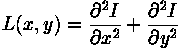



This can be calculated using a

convolution
filter.

Since the input image is represented as a set of discrete pixels, we have to find a discrete convolution kernel that can approximate the second derivatives in the definition of the Laplacian. Two commonly used small kernels are shown in Figure 1.



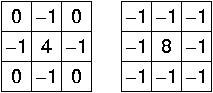
Figure 1 Two commonly used discrete approximations to the Laplacian filter. (Note, we have defined the Laplacian using a negative peak because this is more common; however, it is equally valid to use the opposite sign convention.)

Using one of these kernels, the Laplacian can be calculated using standard convolution methods.

Because these kernels are approximating a second derivative measurement on the image, they are very sensitive to noise. To counter this, the image is oftenGaussian
smoothed before applying the Laplacian filter. This pre-processing step reduces the high frequency noise components prior to the differentiation step.

In fact, since the convolution operation is associative, we can convolve the Gaussian smoothing filter with the Laplacian filter first of all, and then convolve this hybrid filter with the image to achieve the required result. Doing things this way has two
advantages:

Since both the Gaussian and the Laplacian kernels are usually much smaller than the image, this method usually requires far fewer arithmetic operations.

The LoG (`Laplacian of Gaussian') kernel can be precalculated in advance so only one convolution needs to be performed at run-time on the image.

The 2-D LoG function centered on zero and with Gaussian standard deviation

has the form:



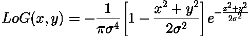
and is shown in Figure 2.



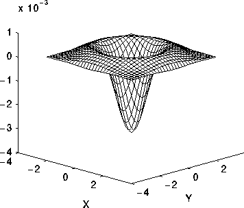
Figure 2 The 2-D Laplacian of Gaussian (LoG) function. The x and y axes are marked in standard deviations (

).

A discrete kernel that approximates this function (for a Gaussian

= 1.4) is shown in Figure 3.



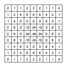
Figure 3 Discrete approximation to LoG function with Gaussian

= 1.4

Note that as the Gaussian is made increasingly narrow, the LoG kernel becomes the same as the simple Laplacian kernels shown in Figure 1. This is because smoothing with a very narrow Gaussian (

<
0.5 pixels) on a discrete grid has no effect. Hence on a discrete grid, the simple Laplacian can be seen as a limiting case of the LoG for narrow Gaussians.

Guidelines for Use

The LoG operator calculates the second spatial derivative of an image. This means that in areas where the image has a constant intensity (i.e. where the intensity gradient is zero), the LoG response will be zero. In the vicinity of a change in intensity,
however, the LoG response will be positive on the darker side, and negative on the lighter side. This means that at a reasonably sharp edge between two regions of uniform but different intensities, the LoG response will be:

zero at a long distance from the edge,
positive just to one side of the edge,
negative just to the other side of the edge,
zero at some point in between, on the edge itself.

Figure 4 illustrates the response of the LoG to a step edge.



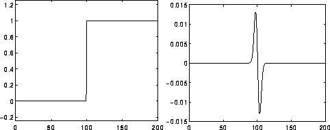
Figure 4 Response of 1-D LoG filter to a step edge. The left hand graph shows a 1-D image, 200 pixels long, containing a step edge. The right hand graph shows the response of a 1-D LoG filter with Gaussian

=
3 pixels.

By itself, the effect of the filter is to highlight edges in an image.

For example,





is a simple image with strong edges.

The image





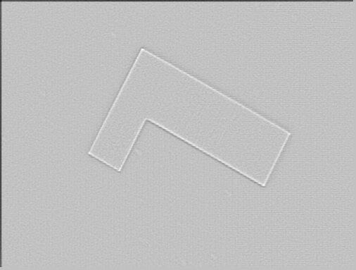
is the result of applying a LoG filter with Gaussian

= 1.0. A 7×7 kernel was used. Note that the output contains negative
and non-integer values, so for display purposes the image has been normalized to the range 0 - 255.


If a portion of the filtered, or gradient, image is added to
the original image, then the result will be to make any edges in the original image much sharper and give them more contrast. This is commonly used as an enhancement technique in remote sensing applications.

To see this we start with





which is a slightly blurry image of a face.

The image





is the effect of applying an LoG filter with Gaussian

= 1.0, again using a 7×7 kernel.

Finally,





is the result of combining (i.e. subtracting) the filtered image and the original image. Note that
the filtered image had to be suitable scaled before combining in order to produce a sensible enhancement.
Also, it may be necessary to translate the filtered image by half the width of the convolution kernel in
both the x and y directions in order to register the images correctly.

The enhancement has made edges sharper but has also increased the effect of noise. If we simply filter the image with a Laplacian (i.e. use a LoG filter with a very narrow Gaussian) we obtain





Performing edge enhancement using this sharpening image yields the noisy result





(Note that unsharp filtering may produce an equivalent result since it can be defined by adding the
negative Laplacian image (or any suitable edge image) onto the original.) Conversely, widening the Gaussian smoothing component of the operator can reduce some of this noise, but, at the same time, the enhancement effect becomes less pronounced.

The fact that the output of the filter passes through zero at edges can be used to detect those edges. See the section on zero
crossing edge detection.

Note that since the LoG is an

isotropic
filter, it is not possible to directly extract edge orientation information from the LoG output in the same way that it is for other edge detectors such as the Roberts
Cross and Sobel operators.

Convolving with a kernel such as the one shown in Figure 3 can very easily produce output pixel values that are much larger than any of the input pixels values, and which may be negative. Therefore it is important to use an image type (e.g. floating
point) that supports negative numbers and a large range in order to avoid overflow or saturation. The kernel can also be scaled down by a constant factor in order to reduce the range of output values.

Common Variants

It is possible to approximate the LoG filter with a filter that is just the difference of two differently sized Gaussians. Such a filter is known as a

DoGfilter
(short for

`Difference of Gaussians').

As an aside it has been suggested (Marr 1982) that LoG filters (actually DoG filters) are important in biological visual processing.

An even cruder approximation to the LoG (but much faster to compute) is the DoB filter (

`Difference
of Boxes'). This is simply the difference between twomean filters of different sizes. It produces a kind of squared-off
approximate version of the LoG.

Interactive Experimentation

You can interactively experiment with the Laplacian operator by clicking here.

You can interactively experiment with the Laplacian of Gaussian operator by clicking here.

Exercises

Try the effect of LoG filters using different width Gaussians on the image



What is the general effect of increasing the Gaussian width? Notice particularly the effect on features of different sizes and thicknesses.

Construct a LoG filter where the kernel size is much too small for the chosen Gaussian width (i.e. the LoG becomes truncated). What is the effect on the output? In particular what do you notice about the LoG output in different regions each of
uniform but different intensities?

Devise a rule to determine how big an LoG kernel should be made in relation to the

of the underlying Gaussian if
severe truncation is to be avoided.

If you were asked to construct an edge detector that simply looked for peaks (both positive and negative) in the output from an LoG filter, what would such a detector produce as output from a single step edge?

References

R. Haralick and L. Shapiro Computer and Robot Vision, Vol. 1, Addison-Wesley Publishing Company, 1992, pp 346 - 351.

B. Horn Robot Vision, MIT Press, 1986, Chap. 8.

D. Marr Vision, Freeman, 1982, Chap. 2, pp 54 - 78.

D. Vernon Machine Vision, Prentice-Hall, 1991, pp 98 - 99, 214.

Local Information

Specific information about this operator may be found here.

More general advice about the local HIPR installation is available in the Local Information introductory
section.

DoG (Difference of Gaussian)是灰度图像增强和角点检测的方法，其做法较简单，证明较复杂，具体讲解如下:

Difference of Gaussian(DOG)是高斯函数的差分。我们已经知道可以通过将图像与高斯函数进行卷积得到一幅图像的低通滤波结果，即去噪过程，这里的Gaussian和高斯低通滤波器的高斯一样，是一个函数，即为正态分布函数。



那么difference of Gaussian 即高斯函数差分是两幅高斯图像的差，

一维表示：


二维表示：


具体到图像处理来讲，就是将两幅图像在不同参数下的高斯滤波结果相减，得到DoG图。

1. 处理一幅图像在不同参数下的DoG

[cpp] view
plaincopy

A = Process(Im, 0.3, 0.4, x);

B = Process(Im, 0.6, 0.7, x);

a = getExtrema(A, B, C, thresh);

其中，

[cpp] view
plaincopy

function [ out_img ] = Process( img, sig1, sig2, size )

是求图像DoG的结果，两个高斯平滑参数分别为sig1和sig2,结果如下：

[cpp] view
plaincopy

A = Process(Im, 0.3, 0.4, x);



[cpp] view
plaincopy

B = Process(Im, 0.6, 0.7, x);



[cpp] view
plaincopy

C = Process(Im, 0.7, 0.8, x);



2. 根据DOG求角点

Theory：DOG三维图中的最大值和最小值点是角点



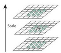
X标记当前像素点，绿色的圈标记邻接像素点，用这个方式，最多检测26个像素点。X被标记为特征点，如果它是所有邻接像素点的最大值或最小值点。

因此在上一步计算出的A,B,C三个DOG图中求图B中是极值的点，并标记（max:1;min:-1）

[cpp] view
plaincopy

a = getExtrema(A, B, C, thresh);

figure;

imshow(a, [-1 1]);

[cpp] view
plaincopy



结果：

黑色为极小值，白色为极大值



最后在原图上予以显示：



就得到了一幅图的DOG角点检测结果。

代码下载链接：http://download.csdn.net/detail/abcjennifer/4363144