深度学习基础(六)Self-Taught Learning 分类: 深度学习 2015-03-20 14:55 24人阅读 评论(0) 收藏
2015-03-20 14:55
176 查看
要想提高学习类的算法,最简单的方法就是使用更多的数据,但是有标签的数据往往是很难获取的,因此对于无标签的数据的学习,我们有自学习算法和无监督特学习算法。
有两类常用的特征学习算法,自学习算法的前提假设是无标签的数据和有标签的数据不一定满足一样的分布,而无监督学习算法的前提假设是两者的分布是一样的。
我们先来介绍一下特征学习:
我们之前讲过自编码器,输入时有标签的数据集
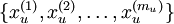
对于训练好的参数:
,给定任意输入,我们可以得到隐层的a。
我们去掉稀疏自编码器的最后一层,就得到如下模型
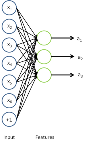
对于每一个输入值

,我们可以得到对应的激活函数

,即如下:

我们的输入可以替换为

,什么意思,实际上是对x进行的特征提取,以提取后的特征作为输入值,这样大大节约了存储空间和计算时间。
练习:
有两类常用的特征学习算法,自学习算法的前提假设是无标签的数据和有标签的数据不一定满足一样的分布,而无监督学习算法的前提假设是两者的分布是一样的。
我们先来介绍一下特征学习:
我们之前讲过自编码器,输入时有标签的数据集
对于训练好的参数:
,给定任意输入,我们可以得到隐层的a。
我们去掉稀疏自编码器的最后一层,就得到如下模型
对于每一个输入值
,我们可以得到对应的激活函数
,即如下:
我们的输入可以替换为
,什么意思,实际上是对x进行的特征提取,以提取后的特征作为输入值,这样大大节约了存储空间和计算时间。
练习:
%% CS294A/CS294W Self-taught Learning Exercise

%  Instructions
%  ------------
%
%  This file contains code that helps you get started on the
%  self-taught learning. You will need to complete code in feedForwardAutoencoder.m
%  You will also need to have implemented sparseAutoencoderCost.m and
%  softmaxCost.m from previous exercises.
%
%% ======================================================================
%  STEP 0: Here we provide the relevant parameters values that will
%  allow your sparse autoencoder to get good filters; you do not need to
%  change the parameters below.

inputSize  = 28 * 28;
numLabels  = 5;
hiddenSize = 200;
sparsityParam = 0.1; % desired average activation of the hidden units.
% (This was denoted by the Greek alphabet rho, which looks like a lower-case "p",
%  in the lecture notes).
lambda = 3e-3;       % weight decay parameter
beta = 3;            % weight of sparsity penalty term
maxIter = 400;

%% ======================================================================
%  STEP 1: Load data from the MNIST database
%
%  This loads our training and test data from the MNIST database files.
%  We have sorted the data for you in this so that you will not have to
%  change it.

% Load MNIST database files
mnistData   = loadMNISTImages('mnist/train-images-idx3-ubyte');
mnistLabels = loadMNISTLabels('mnist/train-labels-idx1-ubyte');

% Set Unlabeled Set (All Images)

% Simulate a Labeled and Unlabeled set
labeledSet   = find(mnistLabels >= 0 & mnistLabels <= 4);
unlabeledSet = find(mnistLabels >= 5);

numTrain = round(numel(labeledSet)/2);
trainSet = labeledSet(1:numTrain);
testSet  = labeledSet(numTrain+1:end);

unlabeledData = mnistData(:, unlabeledSet);

trainData   = mnistData(:, trainSet);
trainLabels = mnistLabels(trainSet)' + 1; % Shift Labels to the Range 1-5

testData   = mnistData(:, testSet);
testLabels = mnistLabels(testSet)' + 1;   % Shift Labels to the Range 1-5

% Output Some Statistics
fprintf('# examples in unlabeled set: %d\n', size(unlabeledData, 2));
fprintf('# examples in supervised training set: %d\n\n', size(trainData, 2));
fprintf('# examples in supervised testing set: %d\n\n', size(testData, 2));

%% ======================================================================
%  STEP 2: Train the sparse autoencoder
%  This trains the sparse autoencoder on the unlabeled training
%  images.

theta = initializaParameters(hiddenSize, inputSize);

%  Randomly initialize the parameters
theta = initializeParameters(hiddenSize, inputSize);

%% ----------------- YOUR CODE HERE ----------------------
%  Find opttheta by running the sparse autoencoder on
%  unlabeledTrainingImages

pottheta = theta;
addpath minFunc/
options.Method = 'lbfgs';
options.maxIter = 400;
options.display = 'on';
[opttheta, loss] = minFunc( @(p) sparseAutoencoderLoss(p, ...
inputSize, hiddenSize, ...
lambda, sparsityParam, ...
beta, unlabeledData), ...
theta, options);

%% -----------------------------------------------------

% Visualize weights
W1 = reshape(opttheta(1:hiddenSize * inputSize), hiddenSize, inputSize);
display_network(W1');

%%======================================================================
%% STEP 3: Extract Features from the Supervised Dataset
%
%  You need to complete the code in feedForwardAutoencoder.m so that the
%  following command will extract features from the data.

trainFeatures = feedForwardAutoencoder(opttheta, hiddenSize, inputSize, ...
trainData);

testFeatures = feedForwardAutoencoder(opttheta, hiddenSize, inputSize, ...
testData);

%%======================================================================
%% STEP 4: Train the softmax classifier

softmaxModel = struct;
%% ----------------- YOUR CODE HERE ----------------------
%  Use softmaxTrain.m from the previous exercise to train a multi-class
%  classifier.

%  Use lambda = 1e-4 for the weight regularization for softmax

% You need to compute softmaxModel using softmaxTrain on trainFeatures and
% trainLabels

lambda = 1e-4;
inputSize = hiddenSize;
numClasses = numel(unique(trainLabels));

options.maxIter = 100;
softmaxModel = softmaxTrain(inputSize, numClasses, lambda, ...
trainFeatures, trainLabels, options);

%% -----------------------------------------------------

%%======================================================================
%% STEP 5: Testing

%% ----------------- YOUR CODE HERE ----------------------
% Compute Predictions on the test set (testFeatures) using softmaxPredict
% and softmaxModel

[pred] = softmaxPredict(softmaxModel, testFeatures);

%% -----------------------------------------------------

% Classification Score
fprintf('Test Accuracy: %f%%\n', 100*mean(pred(:) == testLabels(:)));

% (note that we shift the labels by 1, so that digit 0 now corresponds to
%  label 1)
%
% Accuracy is the proportion of correctly classified images
% The results for our implementation was:
%
% Accuracy: 98.3%
%
%
function [activation] = feedForwardAutoencoder(theta, hiddenSize, visibleSize, data) % theta: trained weights from the autoencoder % visibleSize: the number of input units (probably 64) % hiddenSize: the number of hidden units (probably 25) % data: Our matrix containing the training data as columns. So, data(:,i) is the i-th training example. % We first convert theta to the (W1, W2, b1, b2) matrix/vector format, so that this % follows the notation convention of the lecture notes. W1 = reshape(theta(1:hiddenSize*visibleSize), hiddenSize, visibleSize); b1 = theta(2*hiddenSize*visibleSize+1:2*hiddenSize*visibleSize+hiddenSize); %% ---------- YOUR CODE HERE -------------------------------------- % Instructions: Compute the activation of the hidden layer for the Sparse Autoencoder. activation = sigmoid(W1*data + repmat(b1, [1,size(data,2)])); %------------------------------------------------------------------- end %------------------------------------------------------------------- % Here's an implementation of the sigmoid function, which you may find useful % in your computation of the costs and the gradients. This inputs a (row or % column) vector (say (z1, z2, z3)) and returns (f(z1), f(z2), f(z3)). function sigm = sigmoid(x) sigm = 1 ./ (1 + exp(-x)); end

相关文章推荐
- 深度学习基础(七)Self-Taught Learning to Deep Networks 分类: 深度学习 2015-03-20 21:27 36人阅读 评论(0) 收藏
- Search a 2D Matrix 分类: Leetcode(查找) 2015-04-11 10:19 24人阅读 评论(0) 收藏
- 常用数据库 JDBC URL 格式 分类: Java 2011-01-19 14:55 21582人阅读 评论(1) 收藏 举报 jdbcurl数据库teradatasqlservermicroso
- 深度学习基础(三)(稀疏)自编码器 分类: 深度学习 2015-01-20 15:19 96人阅读 评论(0) 收藏
- 图像处理------移动模糊 分类: 视频图像处理 2015-07-24 09:33 26人阅读 评论(0) 收藏
- 系统学习深度学习(七)--主流深度学习开源框架对比 2017-01-23 11:05 2292人阅读 评论(0) 收藏 举报 分类: 深度学习(30) 目录(?)[+] 转自:http://b
- sgu 208 分类: sgu templates 2015-06-17 01:40 24人阅读 评论(0) 收藏
- FFMPEG:H264解码-SDL显示(RGB32、RGB24、YUV420P、YUV422) 分类: DirectX ffmpeg-SDL-VLC-Live555 VC++ 2014-11-25 17:45 726人阅读 评论(0) 收藏
- sgu220&sgu221 分类: sgu 2015-06-15 22:01 24人阅读 评论(0) 收藏
- 深度学习基础(五)Softmax Regression 分类: 深度学习 2015-02-28 10:28 42人阅读 评论(0) 收藏
- vim配置 分类: Linux 2015-06-18 07:49 24人阅读 评论(0) 收藏
- 视频播放的基本原理 分类: arm-linux-Ubuntu 2015-03-20 11:58 419人阅读 评论(0) 收藏
- 图像处理------简单数字水印 - 文字轧花效果 分类: 视频图像处理 2015-07-24 09:37 24人阅读 评论(0) 收藏
- 深度学习基础(一)神经网络 分类: 深度学习 2015-01-19 21:29 84人阅读 评论(0) 收藏
- leetCode(24):Binary Search Tree Iterator 分类: leetCode 2015-06-23 11:50 192人阅读 评论(0) 收藏
- 【图片压缩】使用canvas,html5进行图片压缩 分类: canvas 图片压缩 压缩 HTML5 fileReader 2015-03-20 17:14 118人阅读 评论(0) 收藏
- WPF设置控件的透明度、背景色 分类: .NET 2012-05-28 14:55 6035人阅读 评论(0) 收藏
- 图像处理--------应用卷积– 轧花与边缘检测 分类: 视频图像处理 2015-07-24 09:50 24人阅读 评论(0) 收藏
- 图像处理------基于阈值模糊 分类: 视频图像处理 2015-07-24 14:49 31人阅读 评论(0) 收藏
- 【canvas马赛克效果】根据加载的图片动态生成对应的马赛克图片 分类: javascript 马赛克效果 马赛克 2015-03-20 17:35 79人阅读 评论(0) 收藏