图像分割必备知识点 | Dice损失 理论+代码

本文包含代码案例和讲解，建议收藏，也顺便点个赞吧。欢迎各路朋友爱好者加我的微信讨论问题：cyx645016617.

在很多关于医学图像分割的竞赛、论文和项目中，发现 Dice 系数(Dice coefficient) 损失函数出现的频率较多，这里整理一下。使用图像分割，绕不开Dice损失，这个就好比在目标检测中绕不开IoU一样。

1 概述

Dice损失和Dice系数（Dice coefficient）是同一个东西，他们的关系是：

### 1.2 Dice 定义 - Dice系数, 根据 Lee Raymond Dice命名，是一种**集合相似度度量函数**，通常用于计算两个样本的相似度(值范围为 [0, 1])。 $$DiceCoefficient = \frac{2|X \bigcap Y|}{|X| + |Y|}$$ 其中$|X| \bigcap |Y|$表示X和Y集合的交集，|X|和|Y|表示其元素个数，**对于分割任务而言，|X|和|Y|表示分割的ground truth和predict_mask**。 此外，**我们可以得到Dice Loss的公式：** $$DiceLoss = 1- \frac{2|X \bigcap Y|}{|X| + |Y|}$$ ## 2 手推案例 这个Dice网上有一个非常好二分类的Dice Loss的手推的案例，非常好理解，过程分成两个部分： 1. 先计算$|X|\bigcap|Y|$ 2. 再计算$|X|$和$|Y|$ 计算loss我们必然已经有了这两个参数，模型给出的output，也就是预测的mask；数据集中的ground truth（GT），也就是真实的mask。 在很多关于医学图像分割的竞赛、论文和项目中，发现 Dice 系数(Dice coefficient) 损失函数出现的频率较多，这里整理一下。**使用图像分割，绕不开Dice损失，这个就好比在目标检测中绕不开IoU一样**。 ## 1 概述 Dice损失和Dice系数（Dice coefficient）是同一个东西，他们的关系是： $$DiceLoss = 1-DiceCoefficient$$ ### 1.2 Dice 定义 - Dice系数, 根据 Lee Raymond Dice命名，是一种**集合相似度度量函数**，通常用于计算两个样本的相似度(值范围为 [0, 1])。 $$DiceCoefficient = \frac{2|X \bigcap Y|}{|X| + |Y|}$$ 其中$|X| \bigcap |Y|$表示X和Y集合的交集，|X|和|Y|表示其元素个数，**对于分割任务而言，|X|和|Y|表示分割的ground truth和predict_mask**。 此外，**我们可以得到Dice Loss的公式：** $$DiceLoss = 1- \frac{2|X \bigcap Y|}{|X| + |Y|}$$ ## 2 手推案例 这个Dice网上有一个非常好二分类的Dice Loss的手推的案例，非常好理解，过程分成两个部分： 1. 先计算$|X|\bigcap|Y|$ 2. 再计算$|X|$和$|Y|$ 计算loss我们必然已经有了这两个参数，模型给出的output，也就是预测的mask；数据集中的ground truth（GT），也就是真实的mask。 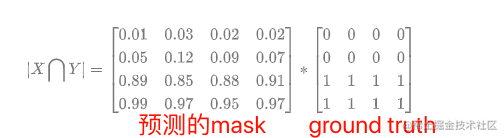 当然还没完，还要把结果加和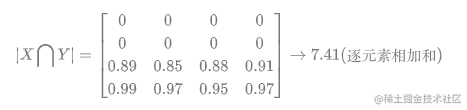：  对于二分类问题，GT分割图是只有 0, 1 两个值的，因此可以有效的将在 Pred 分割图中未在 GT 分割图中激活的所有像素清零. 对于激活的像素，主要是惩罚低置信度的预测，较高值会得到更好的 Dice 系数. 关于计算$|X|$和$|Y|$，如下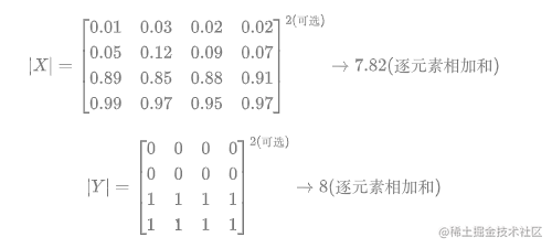：  **其中需要注意的是，一半情况下，这个是直接对所有元素求和，当然有对所有元素先平方再求和的做法。总之就这么多，非常的简单好用。不过上面的内容是针对分割二分类的情况，对于多分类的情况和二分类基本相同**。 ## 3 二分类代码实现 在实现的时候，往往会加上一个smooth，防止分母为0的情况出现。所以公式变成： $$DiceLoss = 1- \frac{2|X \bigcap Y|+smooth}{|X| + |Y|+smooth}$$ **一般smooth为1** ### 3.1 PyTorch实现 先是dice coefficient的实现，pred和target的shape为【batch_size,channels,...】,2D和3D的都可以用这个。 ```python def dice_coeff(pred, target): smooth = 1. num = pred.size(0) m1 = pred.view(num, -1) # Flatten m2 = target.view(num, -1) # Flatten intersection = (m1 * m2).sum() return (2. * intersection + smooth) / (m1.sum() + m2.sum() + smooth) ``` 当然dice loss就是1-dice ceofficient，所以可以写成： ```python def dice_coeff(pred, target): smooth = 1. num = pred.size(0) m1 = pred.view(num, -1) # Flatten m2 = target.view(num, -1) # Flatten intersection = (m1 * m2).sum() return 1-(2. * intersection + smooth) / (m1.sum() + m2.sum() + smooth) ``` ### 3.2 keras实现 ```python smooth = 1. # 用于防止分母为0. def dice_coef(y_true, y_pred): y_true_f = K.flatten(y_true) # 将 y_true 拉伸为一维. y_pred_f = K.flatten(y_pred) intersection = K.sum(y_true_f * y_pred_f) return (2. * intersection + smooth) / (K.sum(y_true_f * y_true_f) + K.sum(y_pred_f * y_pred_f) + smooth) def dice_coef_loss(y_true, y_pred): return 1. - dice_coef(y_true, y_pred) ``` ### 3.3 tensorflow实现 ```python def dice_coe(output, target, loss_type='jaccard', axis=(1, 2, 3), smooth=1e-5): """ Soft dice (Sørensen or Jaccard) coefficient for comparing the similarity of two batch of data, usually be used for binary image segmentation i.e. labels are binary. The coefficient between 0 to 1, 1 means totally match. Parameters ----------- output : Tensor A distribution with shape: [batch_size, ....], (any dimensions). target : Tensor The target distribution, format the same with `output`. loss_type : str ``jaccard`` or ``sorensen``, default is ``jaccard``. axis : tuple of int All dimensions are reduced, default ``[1,2,3]``. smooth : float This small value will be added to the numerator and denominator. - If both output and target are empty, it makes sure dice is 1. - If either output or target are empty (all pixels are background), dice = ```smooth/(small_value + smooth)``, then if smooth is very small, dice close to 0 (even the image values lower than the threshold), so in this case, higher smooth can have a higher dice. Examples --------- >>> outputs = tl.act.pixel_wise_softmax(network.outputs) >>> dice_loss = 1 - tl.cost.dice_coe(outputs, y_) References ----------- - `Wiki-Dice <https://en.wikipedia.org/wiki/Sørensen–Dice_coefficient>`__ """ inse = tf.reduce_sum(output * target, axis=axis) if loss_type == 'jaccard': l = tf.reduce_sum(output * output, axis=axis) r = tf.reduce_sum(target * target, axis=axis) elif loss_type == 'sorensen': l = tf.reduce_sum(output, axis=axis) r = tf.reduce_sum(target, axis=axis) else: raise Exception("Unknow loss_type") dice = (2. * inse + smooth) / (l + r + smooth) dice = tf.reduce_mean(dice) return dice ``` ## 4 多分类 假设是一个10分类的任务，那么我们应该会有一个这样的模型预测结果：[batch_size,10,width,height]，然后我们的ground truth需要改成one hot的形式，也变成[batch_size,10,width,height]。剩下的和二分类的代码基本相同了，先ground truth和预测结果对应元素相乘，然后对相乘的结果求和。就是最后需要对每一个类别和每一个样本都求一次平均就行了。 ## 5 深入探讨Dice，IoU 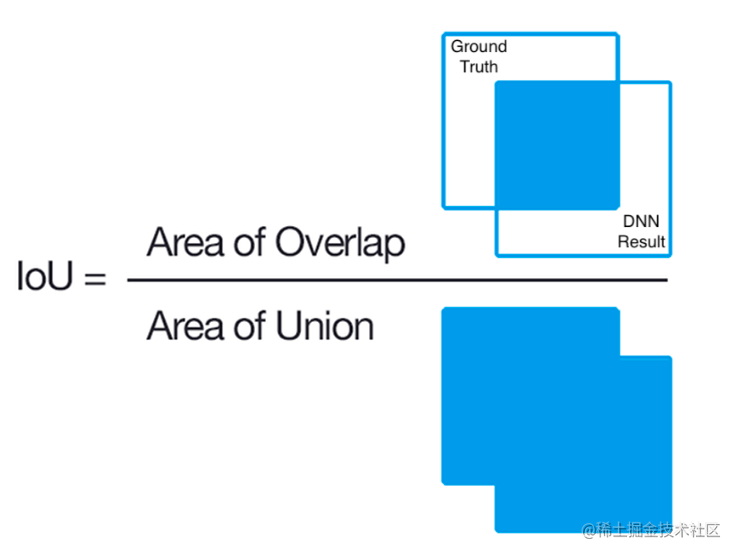 上图就是我们常见的IoU方法，假设分子的两个集合，一个集合是Ground Truth，另外一个集合是神经网络给出的预测值。**不要被图中的正方形的形状限制了想想，对于分割任务来说，一般是像素级的不规则图案**。 如果预测正确，也就是分子中的蓝色交汇的部分，称之为True Positive，属于True Positive的像素的数量就是分子的值。分母的值是Ground Truth的所有像素的数量和预测结果中所有像素的数量的和再减去重叠的部分的像素数量。 直接学过recall，precision，混淆矩阵，f1score的朋友一定对FN，TP，TN，FP这些不陌生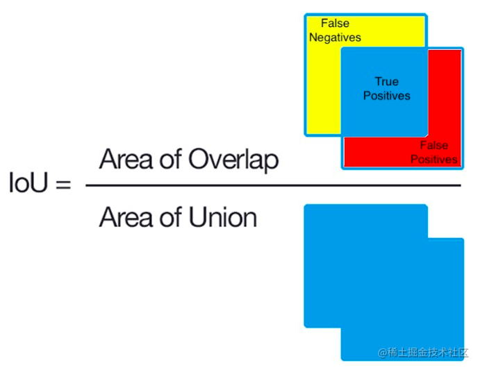：  - 黄色区域：预测为negative，但是GT中是positive的False Negative区域； - 红色区域：预测为positive，但是GT中是Negative的False positive区域； 对于IoU的预测好坏的直观理解就是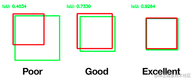：  **简单的说就是，重叠的越多，IoU越接近1，预测效果越好**。 现在让我们更好的从IoU过渡到Dice，我们先把IoU的算式写出来： $$IoU = \frac{TP}{TP+FP+FN}$$ Dice的算式，结合我们之前讲的内容，可以推导出，$|X|\bigcap|Y|$就是TP，$|X|$假设是GT的话就是FN+TP，$|Y|$假设是预测的mask，就是TP+FP，所以： $$Dice_coefficient = \frac{2\times TP}{TP+FN + TP + FP}$$ 所以我们可以得到Dice和IoU之间的关系了，**这里的之后的Dice默认表示Dice Coefficient**： $$IoU = \frac{Dice}{2-Dice}$$ 这个函数图像如下图，我们只关注0～1这个区间就好了，可以发现： - IoU和Dice同时为0，同时为1；这很好理解，就是全预测正确和全部预测错误 - 假设在相同的预测情况下，可以发现Dice给出的评价会比IoU高一些，哈哈哈。**所以Dice的数据会更加好看一些。** 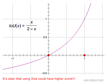 参考文章： 1. https://www.aiuai.cn/aifarm1159.html 2. https://blog.csdn.net/py184473894/article/details/90383618