动手学深度学习 Task04 机器翻译及相关技术；注意力机制与Seq2seq模型；Transformer

【一】机器翻译及相关技术

• 机器翻译（MT）：
  将一段文本从一种语言自动翻译为另一种语言，用神经网络解决这个问题通常称为神经机器翻译（NMT）。 主要特征：输出的是单词序列而不是单个单词。 输出序列的长度可能与源序列的长度不同。
• 数据预处理
  将数据集清洗、转化为神经网络的输入minbatch。字符在计算机里是以编码的形式存在，我们通常所用的空格是 \x20 ，是在标准ASCII可见字符 0x20~0x7e 范围内。 而 \xa0 属于 latin1 （ISO/IEC_8859-1）中的扩展字符集字符，代表不间断空白符nbsp(non-breaking space)，超出gbk编码范围，是需要去除的特殊字符。所以在数据预处理的过程中，首先需要对数据进行清洗。
• 分词
  字符串—单词组成的列表
• 建立词典
  单词组成的列表—单词id组成的列表

#测试
def translate_ch7(model, src_sentence, src_vocab, tgt_vocab, max_len, device):
src_tokens = src_vocab[src_sentence.lower().split(' ')]
src_len = len(src_tokens)
if src_len < max_len:
src_tokens += [src_vocab.pad] * (max_len - src_len)
enc_X = torch.tensor(src_tokens, device=device)
enc_valid_length = torch.tensor([src_len], device=device)
# use expand_dim to add the batch_size dimension.
enc_outputs = model.encoder(enc_X.unsqueeze(dim=0), enc_valid_length)
dec_state = model.decoder.init_state(enc_outputs, enc_valid_length)
dec_X = torch.tensor([tgt_vocab.bos], device=device).unsqueeze(dim=0)
predict_tokens = []
for _ in range(max_len):
Y, dec_state = model.decoder(dec_X, dec_state)
# The token with highest score is used as the next time step input.
dec_X = Y.argmax(dim=2)
py = dec_X.squeeze(dim=0).int().item()
if py == tgt_vocab.eos:
break
predict_tokens.append(py)
return ' '.join(tgt_vocab.to_tokens(predict_tokens))
for sentence in ['Go .', 'Wow !', "I'm OK .", 'I won !']:
print(sentence + ' => ' + translate_ch7(
model, sentence, src_vocab, tgt_vocab, max_len, ctx))

Sequence to Sequence模型
模型：

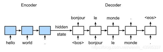
训练

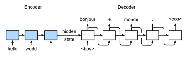
预测

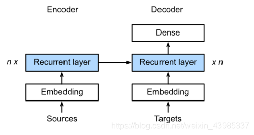
具体结构：

【二】注意力机制与Seq2seq模型
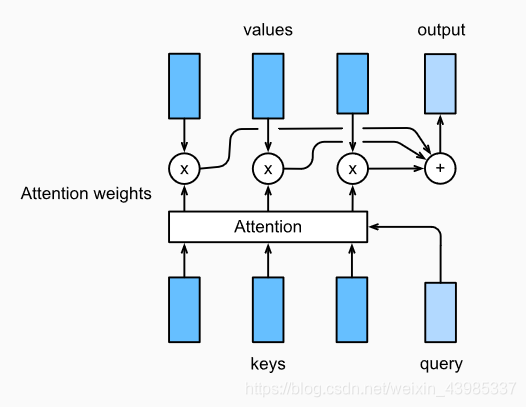
注意力机制框架
Attention 是一种通用的带权池化方法，输入由两部分构成：询问（query）和键值对（key-value pairs）。 Ki∈Rdk,Vi∈RdvK_i∈ℝ^{d_k}, V_i∈ℝ^{d_v}Ki​∈Rdk​,Vi​∈Rdv​. Query q∈Rdqq∈ℝ^{d_q}q∈Rdq​ , attention layer得到输出与value的维度一致 o∈Rdvo∈ℝ^{d_v}o∈Rdv​. 对于一个query来说，attention layer 会与每一个key计算注意力分数并进行权重的归一化，输出的向量 o 则是value的加权求和，而每个key计算的权重与value一一对应。
为了计算输出，我们首先假设有一个函数 α 用于计算query和key的相似性，然后可以计算所有的 attention scores a1,…,ana_1, \ldots, a_na1​,…,an​ by ai=α(q,ki).a_i = \alpha(\mathbf q, \mathbf k_i).ai​=α(q,ki​).我们使用 softmax函数 获得注意力权重：b1,…,bn=softmax(a1,…,an).b_1, \ldots, b_n = \textrm{softmax}(a_1, \ldots, a_n).b1​,…,bn​=softmax(a1​,…,an​).
最终的输出就是value的加权求和：o=∑i=1nbivi.\mathbf o = \sum_{i=1}^n b_i \mathbf v_i.o=i=1∑n​bi​vi​.

不同的attetion layer的区别在于score函数的选择，在本节的其余部分，我们将讨论两个常用的注意层 Dot-product Attention 和 Multilayer Perceptron Attention；随后我们将实现一个引入attention的seq2seq模型并在英法翻译语料上进行训练与测试。
多层感知机注意力
在多层感知器中，我们首先将 query and keys 投影到Rhℝ^ℎRh.为了更具体，我们将可以学习的参数做如下映射Wk∈Rh×dk,Wq∈Rh×dq,and,V∈RhW_k∈ℝ^{ℎ×d_k},W_q∈ℝ^{ℎ×d_q},and, V∈ℝ^hWk​∈Rh×dk​,Wq​∈Rh×dq​,and,V∈Rh. 将score函数定义α(q,k)=vTtanh(Wkk+Wqq)\alpha( \mathbf {q,k}) = \mathbf v^Ttanh( \mathbf {W_kk+W_qq}) α(q,k)=vTtanh(Wk​k+Wq​q)然后将key 和 value 在特征的维度上合并（concatenate），然后送至 a single hidden layer perceptron 这层中 hidden layer 为 ℎ and 输出的size为 1 .隐层激活函数为tanh，无偏置.

# Save to the d2l package.
class MLPAttention(nn.Module):
def __init__(self, units,ipt_dim,dropout, **kwargs):
super(MLPAttention, self).__init__(**kwargs)
# Use flatten=True to keep query's and key's 3-D shapes.
self.W_k = nn.Linear(ipt_dim, units, bias=False)
self.W_q = nn.Linear(ipt_dim, units, bias=False)
self.v = nn.Linear(units, 1, bias=False)
self.dropout = nn.Dropout(dropout)

def forward(self, query, key, value, valid_length):
query, key = self.W_k(query), self.W_q(key)
#print("size",query.size(),key.size())
# expand query to (batch_size, #querys, 1, units), and key to
# (batch_size, 1, #kv_pairs, units). Then plus them with broadcast.
features = query.unsqueeze(2) + key.unsqueeze(1)
#print("features:",features.size())  #--------------开启
scores = self.v(features).squeeze(-1)
attention_weights = self.dropout(masked_softmax(scores, valid_length))
return torch.bmm(attention_weights, value)

测试
尽管MLPAttention包含一个额外的MLP模型，但如果给定相同的输入和相同的键，我们将获得与DotProductAttention相同的输出

atten = MLPAttention(ipt_dim=2,units = 8, dropout=0)
atten(torch.ones((2,1,2), dtype = torch.float), keys, values, torch.FloatTensor([2, 6]))

总结
注意力层显式地选择相关的信息。
注意层的内存由键-值对组成，因此它的输出接近于键类似于查询的值。
引入注意力机制的Seq2seq模型
本节中将注意机制添加到sequence to sequence 模型中，以显式地使用权重聚合states。下图展示encoding 和decoding的模型结构，在时间步为t的时候。此刻attention layer保存着encodering看到的所有信息——即encoding的每一步输出。在decoding阶段，解码器的 t 时刻的隐藏状态被当作query，encoder的每个时间步的hidden states作为key和value进行attention聚合. Attetion model的输出当作成上下文信息context vector，并与解码器输入 DtD_tDt​ 拼接起来一起送到解码器：

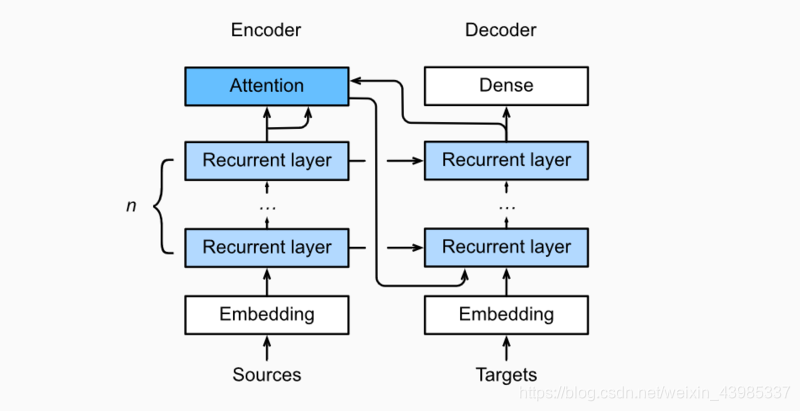Fig1具有注意机制的seq−to−seq模型解码的第二步\qquad Fig1具有注意机制的seq−to−seq模型解码的第二步Fig1具有注意机制的seq−to−seq模型解码的第二步

下图展示了seq2seq机制的所以层的关系，下面展示了encoder和decoder的layer结构
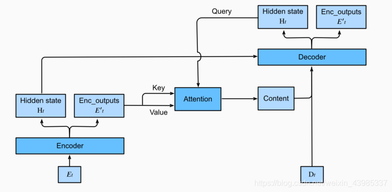Fig2具有注意机制的seq−to−seq模型中层结构\qquad Fig2具有注意机制的seq−to−seq模型中层结构Fig2具有注意机制的seq−to−seq模型中层结构

mport sys
sys.path.append('/home/kesci/input/d2len9900')
import d2li

解码器
由于带有注意机制的seq2seq的编码器与之前章节中的Seq2SeqEncoder相同，所以在此处我们只关注解码器。我们添加了一个MLP注意层(MLPAttention)，它的隐藏大小与解码器中的LSTM层相同。然后我们通过从编码器传递三个参数来初始化解码器的状态:

• the encoder outputs of all timesteps：encoder输出的各个状态，被用于attetion layer的memory部分，有相同的key和values
• the hidden state of the encoder’s final timestep：编码器最后一个时间步的隐藏状态，被用于初始化decoder 的hidden state
• the encoder valid length: 编码器的有效长度，借此，注意层不会考虑编码器输出中的填充标记（Paddings）
  在解码的每个时间步，我们使用解码器的最后一个RNN层的输出作为注意层的query。然后，将注意力模型的输出与输入嵌入向量连接起来，输入到RNN层。虽然RNN层隐藏状态也包含来自解码器的历史信息，但是attention model的输出显式地选择了enc_valid_len以内的编码器输出，这样attention机制就会尽可能排除其他不相关的信息。

class Seq2SeqAttentionDecoder(d2l.Decoder):
def __init__(self, vocab_size, embed_size, num_hiddens, num_layers,
dropout=0, **kwargs):
super(Seq2SeqAttentionDecoder, self).__init__(**kwargs)
self.attention_cell = MLPAttention(num_hiddens,num_hiddens, dropout)
self.embedding = nn.Embedding(vocab_size, embed_size)
self.rnn = nn.LSTM(embed_size+ num_hiddens,num_hiddens, num_layers, dropout=dropout)
self.dense = nn.Linear(num_hiddens,vocab_size)

def init_state(self, enc_outputs, enc_valid_len, *args):
outputs, hidden_state = enc_outputs
#         print("first:",outputs.size(),hidden_state[0].size(),hidden_state[1].size())
# Transpose outputs to (batch_size, seq_len, hidden_size)
return (outputs.permute(1,0,-1), hidden_state, enc_valid_len)
#outputs.swapaxes(0, 1)

def forward(self, X, state):
enc_outputs, hidden_state, enc_valid_len = state
#("X.size",X.size())
X = self.embedding(X).transpose(0,1)
#         print("Xembeding.size2",X.size())
outputs = []
for l, x in enumerate(X):
#             print(f"\n{l}-th token")
#             print("x.first.size()",x.size())
# query shape: (batch_size, 1, hidden_size)
# select hidden state of the last rnn layer as query
query = hidden_state[0][-1].unsqueeze(1) # np.expand_dims(hidden_state[0][-1], axis=1)
# context has same shape as query
#             print("query enc_outputs, enc_outputs:\n",query.size(), enc_outputs.size(), enc_outputs.size())
context = self.attention_cell(query, enc_outputs, enc_outputs, enc_valid_len)
# Concatenate on the feature dimension
#             print("context.size:",context.size())
x = torch.cat((context, x.unsqueeze(1)), dim=-1)
# Reshape x to (1, batch_size, embed_size+hidden_size)
#             print("rnn",x.size(), len(hidden_state))
out, hidden_state = self.rnn(x.transpose(0,1), hidden_state)
outputs.append(out)
outputs = self.dense(torch.cat(outputs, dim=0))
return outputs.transpose(0, 1), [enc_outputs, hidden_state,
enc_valid_len]

现在我们可以用注意力模型来测试seq2seq。为了与第9.7节中的模型保持一致，我们对vocab_size、embed_size、num_hiddens和num_layers使用相同的超参数。结果，我们得到了相同的解码器输出形状，但是状态结构改变了。

encoder = d2l.Seq2SeqEncoder(vocab_size=10, embed_size=8,
num_hiddens=16, num_layers=2)
# encoder.initialize()
decoder = Seq2SeqAttentionDecoder(vocab_size=10, embed_size=8,
num_hiddens=16, num_layers=2)
X = torch.zeros((4, 7),dtype=torch.long)
print("batch size=4\nseq_length=7\nhidden dim=16\nnum_layers=2\n")
print('encoder output size:', encoder(X)[0].size())
print('encoder hidden size:', encoder(X)[1][0].size())
print('encoder memory size:', encoder(X)[1][1].size())
state = decoder.init_state(encoder(X), None)
out, state = decoder(X, state)
out.shape, len(state), state[0].shape, len(state[1]), state[1][0].shape

【三】Transformer
Transformer模型利用attention机制实现了并行化捕捉序列依赖，并且同时处理序列的每个位置的tokens，上述优势使得Transformer模型在性能优异的同时大大减少了训练时间。下图展示了Transformer模型的架构，之前的seq2seq模型相似，Transformer同样基于编码器-解码器架构，其区别主要在于以下三点：

1. Transformer blocks：将seq2seq模型重的循环网络替换为了Transformer Blocks，该模块包含一个多头注意力层（Multi-head Attention Layers）以及两个position-wise feed-forward networks（FFN）。对于解码器来说，另一个多头注意力层被用于接受编码器的隐藏状态。
2. Add and norm：多头注意力层和前馈网络的输出被送到两个“add and norm”层进行处理，该层包含残差结构以及层归一化。
3. Position encoding：由于自注意力层并没有区分元素的顺序，所以一个位置编码层被用于向序列元素里添加位置信息。
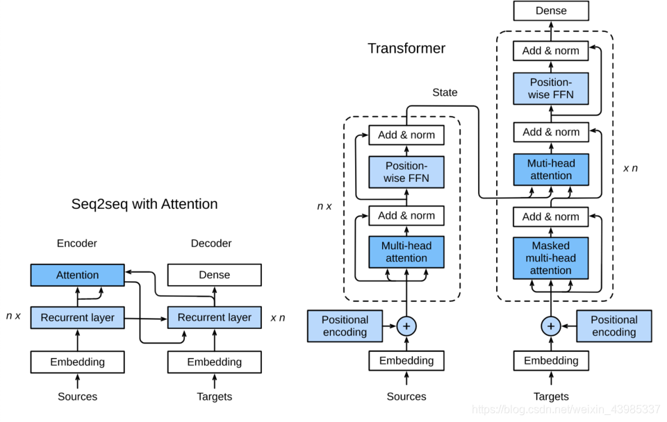   Fig.Transformer架构.\qquad Fig. Transformer架构.Fig.Transformer架构.

位置编码
与循环神经网络不同，无论是多头注意力网络还是前馈神经网络都是独立地对每个位置的元素进行更新，这种特性帮助我们实现了高效的并行，却丢失了重要的序列顺序的信息。为了更好的捕捉序列信息，Transformer模型引入了位置编码去保持输入序列元素的位置。

假设输入序列的嵌入表示 X∈Rl×dX\in \mathbb{R}^{l\times d}X∈Rl×d, 序列长度为 l 嵌入向量维度为 d ，则其位置编码为P∈Rl×dP \in \mathbb{R}^{l\times d}P∈Rl×d，输出的向量就是二者相加 X+PX + PX+P。

位置编码是一个二维的矩阵，i对应着序列中的顺序，j对应其embedding vector内部的维度索引。我们可以通过以下等式计算位置编码：Pi,2j=sin(i/100002j/d)P_{i,2j} = sin(i/10000^{2j/d})Pi,2j​=sin(i/100002j/d)Pi,2j+1=cos(i/100002j/d)P_{i,2j+1} = cos(i/10000^{2j/d})Pi,2j+1​=cos(i/100002j/d)for i=0,…,l−1 and j=0,…,⌊(d−1)/2⌋for\ i=0,\ldots, l-1\ and\ j=0,\ldots,\lfloor (d-1)/2 \rfloorfor i=0,…,l−1 and j=0,…,⌊(d−1)/2⌋

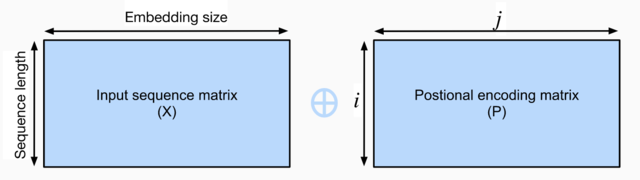
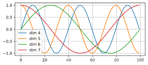
Fig.10.3.4位置编码\qquad Fig.10.3.4 位置编码Fig.10.3.4位置编码

class PositionalEncoding(nn.Module):
def __init__(self, embedding_size, dropout, max_len=1000):
super(PositionalEncoding, self).__init__()
self.dropout = nn.Dropout(dropout)
self.P = np.zeros((1, max_len, embedding_size))
X = np.arange(0, max_len).reshape(-1, 1) / np.power(
10000, np.arange(0, embedding_size, 2)/embedding_size)
self.P[:, :, 0::2] = np.sin(X)
self.P[:, :, 1::2] = np.cos(X)
self.P = torch.FloatTensor(self.P)

def forward(self, X):
if X.is_cuda and not self.P.is_cuda:
self.P = self.P.cuda()
X = X + self.P[:, :X.shape[1], :]
return self.dropout(X)

测试
下面我们用PositionalEncoding这个类进行一个小测试，取其中的四个维度进行可视化。 我们可以看到，第4维和第5维有相同的频率但偏置不同。第6维和第7维具有更低的频率；因此positional encoding对于不同维度具有可区分性。

import numpy as np
pe = PositionalEncoding(20, 0)
Y = pe(torch.zeros((1, 100, 20))).numpy()
d2l.plot(np.arange(100), Y[0, :, 4:8].T, figsize=(6, 2.5),
legend=["dim %d" % p for p in [4, 5, 6, 7]])

注：

• 在Transformer模型中，注意力头数为h，嵌入向量和隐藏状态维度均为d，那么一个多头注意力层所含的参数量是：4hd24hd^24hd2
• 层归一化有利于加快收敛，减少训练时间成本;对一个中间层的所有神经元进行归一化;层归一化的效果不会受到batch大小的影响.

• 点赞
• 收藏
• 分享
• 文章举报