sklearn 套索回归模型和参数选择

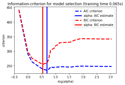
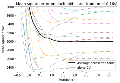
本算例主要验证套索回归中，分别采用AIC,BIC和交叉验证动态调整alpha的值，对结果的影响。
采用AIC、BIC信息标准的模型选择通常十分迅速，但是依赖于对合适的自由度的评价，并且在大数据量的分析中，往往假定模型是正确的，然而基于数据产生的模型去描述事物通常不准确，存在实际特征大于样本的情况。
对于交叉验证，分别采用20层的LassoCV算法和最小角回归算法路径进行计算，又称为并行下降算法，这2种算法得出结果大致相同，不同的是计算速度和数据误差的来源。
最小角回归算法，从结果上来说，在数据特征维度不大时，非常有效，而且计算不需要设定任何初始值。相对来看，并行下降算法（即交叉验证），在一个特定的网络结构中计算（算例中使用的初始值），因此在计算节点数小于特征维度时，效率会很高。因此，在特征维度很大，且数据样本充足的条件下，交叉验证的方法相对于单纯的最小角回归算法，训练误差会更小。
值得注意的是，在针对不确定或不可观测的数据时，模型的选择和参数的设置息息相关。

print(__doc__)

# Author: Olivier Grisel, Gael Varoquaux, Alexandre Gramfort
# License: BSD 3 clause

import time

import numpy as np
import matplotlib.pyplot as plt

from sklearn.linear_model import LassoCV, LassoLarsCV, LassoLarsIC
from sklearn import datasets

diabetes = datasets.load_diabetes()
X = diabetes.data
y = diabetes.target

rng = np.random.RandomState(42)
X = np.c_[X, rng.randn(X.shape[0], 14)]  # add some bad features

# normalize data as done by Lars to allow for comparison
X /= np.sqrt(np.sum(X ** 2, axis=0))

# #############################################################################
# LassoLarsIC: least angle regression with BIC/AIC criterion

model_bic = LassoLarsIC(criterion='bic')
t1 = time.time()  #计时
model_bic.fit(X, y)
t_bic = time.time() - t1
alpha_bic_ = model_bic.alpha_

model_aic = LassoLarsIC(criterion='aic')
model_aic.fit(X, y)
alpha_aic_ = model_aic.alpha_

def plot_ic_criterion(model, name, color):
alpha_ = model.alpha_
alphas_ = model.alphas_
criterion_ = model.criterion_
plt.plot(-np.log10(alphas_), criterion_, '--', color=color,
linewidth=3, label='%s criterion' % name)
plt.axvline(-np.log10(alpha_), color=color, linewidth=3,
label='alpha: %s estimate' % name)
plt.xlabel('-log(alpha)')
plt.ylabel('criterion')

plt.figure()
plot_ic_criterion(model_aic, 'AIC', 'b')
plot_ic_criterion(model_bic, 'BIC', 'r')
plt.legend()
plt.title('Information-criterion for model selection (training time %.3fs)'
% t_bic)

# #############################################################################
# LassoCV: coordinate descent

# Compute paths
print("Computing regularization path using the coordinate descent lasso...")
t1 = time.time()
model = LassoCV(cv=20).fit(X, y)
t_lasso_cv = time.time() - t1

# Display results
m_log_alphas = -np.log10(model.alphas_)

plt.figure()
ymin, ymax = 2300, 3800
plt.plot(m_log_alphas, model.mse_path_, ':')
plt.plot(m_log_alphas, model.mse_path_.mean(axis=-1), 'k',
label='Average across the folds', linewidth=2)
plt.axvline(-np.log10(model.alpha_), linestyle='--', color='k',
label='alpha: CV estimate')

plt.legend()

plt.xlabel('-log(alpha)')
plt.ylabel('Mean square error')
plt.title('Mean square error on each fold: coordinate descent '
'(train time: %.2fs)' % t_lasso_cv)
plt.axis('tight')
plt.ylim(ymin, ymax)

# #############################################################################
# LassoLarsCV: least angle regression

# Compute paths
print("Computing regularization path using the Lars lasso...")
t1 = time.time()
model = LassoLarsCV(cv=20).fit(X, y)
t_lasso_lars_cv = time.time() - t1

# Display results
m_log_alphas = -np.log10(model.cv_alphas_)

plt.figure()
plt.plot(m_log_alphas, model.mse_path_, ':')
plt.plot(m_log_alphas, model.mse_path_.mean(axis=-1), 'k',
label='Average across the folds', linewidth=2)
plt.axvline(-np.log10(model.alpha_), linestyle='--', color='k',
label='alpha CV')
plt.legend()

plt.xlabel('-log(alpha)')
plt.ylabel('Mean square error')
plt.title('Mean square error on each fold: Lars (train time: %.2fs)'
% t_lasso_lars_cv)
plt.axis('tight')
plt.ylim(ymin, ymax)

plt.show()