不加正则项的逻辑回归

数据可视化

需要安装Python的第三方库numpy、matplotlib，安装好后：

import numpy as np
import matplotlib.pyplot as plt

给的数据是TXT文件，因此要读取TXT文件中的数据，将TXT文件中的数据读入列表，定义了函数：

def file2matrix(filename):
fr = open(filename)
numberOfLines = len(fr.readlines())         #get the number of lines in the file
returnMat = np.zeros((numberOfLines,2))        #prepare matrix to return
labeldata = np.zeros((numberOfLines,1))#prepare labels return
fr = open(filename)
index = 0
for line in fr.readlines():
line = line.strip()
listFromLine = line.split(',')
returnMat[index,:] = listFromLine[0:2]
labeldata[index] = int(listFromLine[-1])
index += 1
return returnMat,labeldata

然后可视化数据：

data1mat,labeldata = file2matrix('ex2data1.txt')
fig = plt.figure()
ax = fig.add_subplot(111)
ax.scatter(data1mat[:,0],data1mat[:,1],c=np.array(labeldata),s=15)
plt.show()

Sigmoid函数

import numpy as np
def sigmoid(x):
y = 1/(1+np.exp(-x))
return y

代价函数、梯度以及训练代价函数

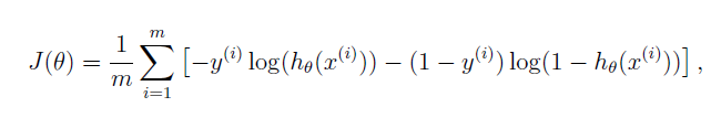
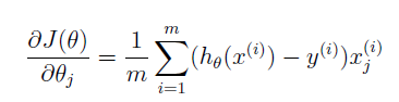
代价函数代码：

import numpy as np
import Sigmoid
def costfunction(theta,X,y):
m = len(y)
J = 0
grad = np.zeros(np.shape(theta))
a = np.dot((-y).reshape(1,m),np.log(Sigmoid.sigmoid(np.dot(X, theta))))
c = (np.ones((m,1))-y).reshape(1,m)
d = np.log(np.ones((m,1))-Sigmoid.sigmoid(np.dot(X,theta)))
b = np.dot(c,d)
J = (a -b)/m
grad = np.dot((Sigmoid.sigmoid(np.dot(X, theta))-y).reshape(1,m),X)/m
grad = grad.reshape(np.shape(theta))
return J,grad

由于吴恩达的课件要求的matlab写作业，所以提供了fminunc的.m函数用于训练代价函数。我不知道这个函数具体 23eb8 是什么，因为我直接使用梯度下降法训练代价函数：

import numpy as np
import plotdata
import CostFunction
X,y = plotdata.file2matrix('ex2data1.txt')
X_shape = np.shape(X)
m = X_shape[0]
n = X_shape[1]
X_1 = np.zeros((m,n+1))
X_1[:,0] = np.ones(m)
X_1[:,1:3] = X
theta = np.zeros((n+1,1))
outloop = 3000
alfa = 0.003
cost_list = np.zeros((int(outloop/100),2))
for i in range(outloop):
cost,grad = CostFunction.costfunction(theta,X_1,y)
theta = theta - alfa*grad
if i%100 == 0:
cost_list[int(i/100),0] = i
cost_list[int(i/100),1] =cost
print(cost,grad,theta)
np.save('theta.npy',theta)

加正则项的逻辑回归

为了更好地拟合我们的数据，我们需要构造新的特征，我们把原先的特征x1、x2构造成：

代码如下：

import file2matrix as f2m
import matplotlib.pyplot as plt
import numpy as np
import costfunctionreg as cfr
from sklearn.preprocessing import PolynomialFeatures
X,y = f2m.file2matrix('ex2data2.txt')
poly = PolynomialFeatures(degree=6, include_bias=False, interaction_only=False)
X_ploly = poly.fit_transform(X)

X_ploly就是我们得到的新的28维的向量，这样我们可以得到更加复杂的决策边界。（ps：这里的函数我在后面的使用都忘了，害得我自己写了一遍mapfeatures函数，看来还是要好好回忆总结啊。）

代价函数、梯度以及训练代价函数

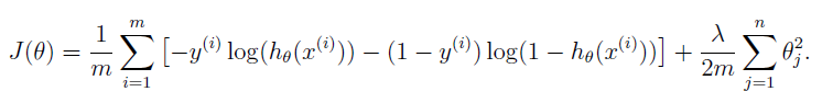
代码实现：

import numpy as np
import Sigmoid
def costfunction(theta,X,y,lamda):
m = len(y)
J = 0
grad = np.zeros(np.shape(theta))
a = np.dot((-y).reshape(1,m),np.log(Sigmoid.sigmoid(np.dot(X, theta))))
c = (np.ones((m,1))-y).reshape(1,m)
d = np.log(np.ones((m,1))-Sigmoid.sigmoid(np.dot(X,theta)))
b = np.dot(c,d)
J = (a -b)/m + lamda * np.dot(np.transpose(theta),theta)/(2*m)
grad = np.dot((Sigmoid.sigmoid(np.dot(X, theta))-y).reshape(1,m),X)/m
grad = grad.reshape(np.shape(theta))
grad = grad + lamda * theta/m
return J,grad

训练代价函数的方法与不加正则项的一样使用梯度下降法。
具体代码：

import file2matrix as f2m
import matplotlib.pyplot as plt
import numpy as np
import costfunctionreg as cfr
from sklearn.preprocessing import PolynomialFeatures
X,y = f2m.file2matrix('ex2data2.txt')
poly = PolynomialFeatures(degree=6, include_bias=False, interaction_only=False)
X_ploly = poly.fit_transform(X)X_shape = np.shape(X_ploly)
m = X_shape[0]
n = X_shape[1]
X_1 = np.zeros((m,n+1))
X_1[:,0] = np.ones(m)
X_1[:,1:m] = X_ploly
theta = np.zeros((n+1,1))
lamda = 1
outloop = 1000000
alfa = 0.003
for i in range(outloop):
cost,grad = cfr.costfunction(theta,X_1,y,lamda)
theta = theta - alfa * grad
print(cost,grad)
np.save('theta.npy',theta)
theta = np.load('theta.npy')
fig = plt.figure()
ax = fig.add_subplot(111)
ax.scatter(X[:,0],X[:,1],c = y,s=15)
plt.figure()
xx = np.arange(0,1.1,0.01).reshape((110,1))
yy = np.arange(0,1.1,0.01).reshape((110,1))
xy = np.hstack((xx,yy))
print(xy.shape)

PS:本人第一次写博客，非常的粗糙，代码也很粗糙，已经是很久之前的代码了，不过就是想总结一下，毕竟年纪大了，学了东西老是忘，最有效的学习方法就是自己再讲出来，将学到的知识输出一遍，更加有利于记忆。

总结

还是要多回忆总结，多学习Python。好了，人生第一篇博客完成！！