Word2Vec词向量模型代码

       Word2Vec也称Word Embedding，中文的叫法是“词向量”或“词嵌入”，是一种计算非常高效的，可以从原始语料中学习字词空间向量的预测模型。Word2Vec可以把一个维数为所有词的数量的高维空间嵌入到一个低维的连续向量空间中，每个单词或词组被映射为实数域上的向量。通过词嵌入这种方式将单词转变为词向量，机器便可对单词进行计算，得到单词之间的相似性。以诗词《全宋词》为训练数据，本文介绍用TensorFlow实现Word2Vec词向量模型的主要代码。

1  读取文件“QuanSongCi.txt”作为训练数据，将文件中的句子转换为词汇列表（英文文本转换为单词列表，中文文本转换为字列表）。

[code]with open('./QuanSongCi.txt', encoding="utf-8") as f:
vocabulary = f.read()
vocabulary = list(vocabulary)

原文：潘阆酒泉子（十之一）长忆钱塘，不是人寰是天上。万家掩映翠微间。处处水潺潺。异花四季当窗放。出入分明在屏障。. . . . . .

文件中句子转换生成的vocabulary词汇表的部分词汇（字）：['潘', '阆', '酒', '泉', '子', '（', '十', '之', '一', '）', '长', '忆', '钱', '塘', '，', '不', '是', '人', '寰',  '是', '天', '上', '。' . .  .]。 

2  生成词汇表字典dictionary和词汇表的反转形式reversed_dictionary。

使用collections.Counter统计词汇列表中词汇的频数，使用most_common 方法取前5000个频数最高的词汇，得到每个词汇的频数统计count。

[code]vocabulary_size = 5000
words = vocabulary
n_words = vocabulary_size - 1
count = [['UNK', -1]]
count.extend(collections.Counter(words).most_common(n_words - 1))

    创建一个字典dictionary，将高频单词放入dictionary中，并按词汇频数排名，为词汇和对应词汇频数的排名：{‘词汇’：排名}。将dictionary的key和value互换生成新的字典reversed_dictionary，即词汇表的反转形式，为词汇频数的排名和对应的词汇：{‘排名’：词汇}。

[code]dictionary = dict()
for word, _ in count:
dictionary[word] = len(dictionary)
reversed_dictionary = dict(zip(dictionary.values(), dictionary.keys()))

  3  使用json模块保存字典dictionary和reversed_dictionary，用于后面的RNN循环神经网络模型训练。

[code]with open("./dictionary.json","w",encoding='utf-8') as f:
json.dump(dictionary,f)
with open("./reverse_dictionary.json","w",encoding='utf-8') as f:
json.dump(reversed_dictionary,f)

 4 定义函数generate_batch(batch_size, num_skips, skip_window)，用来生成训练用的batch和label数据。其中，batch_size是batch的大小，num_skips是对每个单词生成多少个样本，skip_window是单词最远可以联系的距离，设为1代表只能跟紧邻的两个单词生成样本。生成batch和label的主要代码：

[code]for i in range(batch_size // num_skips):
context_words = [w for w in range(span) if w != skip_window]
words_to_use = random.sample(context_words, num_skips)
for j, context_word in enumerate(words_to_use):
batch[i * num_skips + j] = buffer[skip_window]
labels[i * num_skips + j, 0] = buffer[context_word]

 5  建立 Skip-gram模型。

    首先创建graph，并设为默认值graph.as_default()。主要代码：

[code]with tf.device('/cpu:0'):
embeddings = tf.Variable(tf.random_uniform([vocabulary_size, embedding_size], -1.0, 1.0))
embed = tf.nn.embedding_lookup(embeddings, train_inputs)
nce_weights = tf.Variable(tf.truncated_normal([vocabulary_size, embedding_size],
stddev=1.0 / math.sqrt(embedding_size)))
nce_biases = tf.Variable(tf.zeros([vocabulary_size]))
loss = tf.reduce_mean(tf.nn.nce_loss(weights=nce_weights, biases=nce_biases, labels=train_labels,  inputs=embed, num_sampled=num_sampled, num_classes=vocabulary_size))
optimizer = tf.train.GradientDescentOptimizer(1.0).minimize(loss)
similarity = tf.matmul(valid_embeddings, normalized_embeddings, transpose_b=True)

     上述代码中，tf.random_uniform函数随机生成(5000,128)的向量，tf.nn.embedding_lookup函数查找输入train_inputs对应的向量embed，初始化权重参数nce_weigths和偏置nce_biases。用nce_loss函数计算词向量在训练数据上的loss，用tf.train.GradientDescentOptimize函数构建SGD优化器。

    并且计算了embeddings的L2范数norm，用tf.nn.embedding_lookup查询验证单词的嵌入向量，最后计算验证词汇的嵌入向量与词汇表中所有词汇的相似性。

 6  通过函数get_train_data（vocabulary, batch_size, num_steps）获取训练数据batch_inputs和batch_labels，然后用tf.Session.run()开始训练。

[code]with tf.Session(graph=graph) as session:
init.run()
average_loss = 0
for step in range(num_steps):
batch_inputs, batch_labels = generate_batch(batch_size, num_skips, skip_window
feed_dict = {train_inputs: batch_inputs, train_labels: batch_labels}
_, loss_val = session.run([optimizer, loss], feed_dict=feed_dict)
average_loss += loss_val

 输出平均损失average_loss，以及与验证单词相似度最高的8个单词，部分结果如下：

Average loss at step  100000 :  0.9967902089655399

Nearest to 前: 刹, 乡, 峨, 论, 聪, 逊, 棼, 辂,

Nearest to 明: 柳, 是, 万, 处, 十, 放, 一, 几,

Nearest to 空: 品, 鹿, 东, 袜, 像, 谭, 姝, 碑,

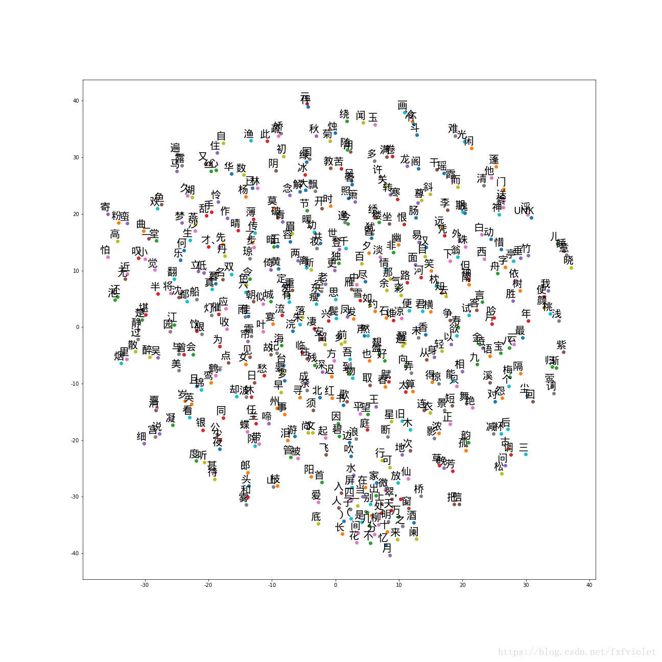
7  可视化词向量效果。定义一个函数def plot_with_labels(low_dim_embs, labels, filename)，其中，low_dim_embs是降维到2维的词汇的空间向量。

[code]def plot_with_labels(low_dim_embs, labels, filename):
assert low_dim_embs.shape[0] >= len(labels)
plt.figure(figsize=(18, 18))
for i, label in enumerate(labels):
x, y = low_dim_embs[i, :]
plt.scatter(x, y)
plt.annotate(label,
xy=(x, y),
xytext=(5, 2),
textcoords='offset points',
ha='right',
va='bottom',
fontproperties=myfont)
plt.savefig(filename)

     下图展示了词频最高的500个单词的可视化结果。 由图可见，意义接近的词，它们的距离比较接近，或者说距离相近的单词在词义上具有较高的相似性。          

版权声明：本文为博主原创文章，转载请注明出处。https://blog.csdn.net/fxfviolet/article/details/82256211