Transform Time Series to Scale/时间序列缩放转换

Like other neural networks, LSTMs expect data to be within the scale of the activation function used by the network.像其他神经网络一样，LSTM希望数据处于网络使用的激活函数的范围内。
The default activation function for LSTMs is the hyperbolic tangent (tanh), which outputs values between -1 and 1. This is the preferred range for the time series data.LSTM的默认激活函数是双曲正切（tanh），它输出-1和1之间的值。这是时间序列数据的首选范围。
To make the experiment fair, the scaling coefficients (min and max) values must be calculated on the training dataset and applied to scale the test dataset and any forecasts. This is to avoid contaminating the experiment with knowledge from the test dataset, which might give the model a small edge.为了使实验公平化，必须在训练数据集上计算缩放系数（最小值和最大值），并将其应用于测试数据集和任何预测的缩放。 这是为了避免被来自测试数据集的知识污染实验，这可能会给模型带来一点小小的优势。（不明白为什么来自测试数据集的所谓‘知识’怎么会污染实验？）
We can transform the dataset to the range [-1, 1] using the MinMaxScaler class. Like other scikit-learn transform classes, it requires data provided in a matrix format with rows and columns. Therefore, we must reshape our NumPy arrays before transforming.我们可以使用MinMaxScaler类将数据集转换为范围[-1，1]。 像其他scikit-learn转换类一样，它需要以行和列格式的矩阵格式数据。 因此，我们必须在转换之前重塑我们的NumPy数组。
For example:

# transform scale
X = series.values
X = X.reshape(len(X), 1)
scaler = MinMaxScaler(feature_range=(-1, 1))
scaler = scaler.fit(X)
scaled_X = scaler.transform(X)

再次，我们必须将预测值的比例反转，将数值返回到原始比例，以便可以解释结果并计算可比较的误差分数。

# invert transform
inverted_X = scaler.inverse_transform(scaled_X)

综合所有这些，下面的例子是洗发水销售数据的缩放转换

rom pandas import read_csv
from pandas import datetime
from pandas import Series
from sklearn.preprocessing import MinMaxScaler
# load dataset
def parser(x):
return datetime.strptime('190'+x, '%Y-%m')
series = read_csv('shampoo-sales.csv', header=0, parse_dates=[0], index_col=0, squeeze=True, date_parser=parser)
print(series.head())
# transform scale
X = series.values
X = X.reshape(len(X), 1)
scaler = MinMaxScaler(feature_range=(-1, 1))
scaler = scaler.fit(X)
scaled_X = scaler.transform(X)
scaled_series = Series(scaled_X[:, 0])
print(scaled_series.head())
# invert transform
inverted_X = scaler.inverse_transform(scaled_X)
inverted_series = Series(inverted_X[:, 0])
print(inverted_series.head())

运行示例，首先打印加载数据的前5行，然后打印缩放数据的前5行，然后打印匹配原始数据的反转缩放的前5行。

Month
1901-01-01    266.0
1901-02-01    145.9
1901-03-01    183.1
1901-04-01    119.3
1901-05-01    180.3

Name: Sales, dtype: float64
0   -0.478585
1   -0.905456
2   -0.773236
3   -1.000000
4   -0.783188
dtype: float64

0    266.0
1    145.9
2    183.1
3    119.3
4    180.3
dtype: float64

现在我们知道如何为LSTM网络准备数据，我们可以开始开发我们的模型了。

总的来说这章槽点不多，MinMaxScaler这个类比较有用

sklearn.preprocessing

.MinMaxScaler

class 

sklearn.preprocessing.

MinMaxScaler

(feature_range=(0, 1), copy=True)[source]

Transforms features by scaling each feature to a given range.This estimator scales and translates each feature individually such that it is in the given range on the training set, i.e. between zero and one.The transformation is given by:[/p]

X_std = (X - X.min(axis=0)) / (X.max(axis=0) - X.min(axis=0))
X_scaled = X_std * (max - min) + min

where min, max = feature_range.This transformation is often used as an alternative to zero mean, unit variance scaling.Read more in the User Guide.

Parameters:

feature_range : tuple (min, max), default=(0, 1) Desired range of transformed data. copy : boolean, optional, default True Set to False to perform inplace row normalization and avoid a copy (if the input is already a numpy array).

Attributes:

min_ : ndarray, shape (n_features,) Per feature adjustment for minimum. scale_ : ndarray, shape (n_features,) Per feature relative scaling of the data. New in version 0.17: scale_ attribute. data_min_ : ndarray, shape (n_features,) Per feature minimum seen in the data New in version 0.17: data_min_ data_max_ : ndarray, shape (n_features,) Per feature maximum seen in the data New in version 0.17: data_max_ data_range_ : ndarray, shape (n_features,) Per feature range  (data_max_ - data_min_)  seen in the data New in version 0.17: data_range_

See also

minmax_scale

Equivalent function without the estimator API.

NotesFor a comparison of the different scalers, transformers, and normalizers, see examples/preprocessing/plot_all_scaling.py.Examples

>>> from sklearn.preprocessing import MinMaxScaler
>>>
>>> data = [[-1, 2], [-0.5, 6], [0, 10], [1, 18]]
>>> scaler = MinMaxScaler()
>>> print(scaler.fit(data))
MinMaxScaler(copy=True, feature_range=(0, 1))
>>> print(scaler.data_max_)
[  1.  18.]
>>> print(scaler.transform(data))
[[ 0.    0.  ]
[ 0.25  0.25]
[ 0.5   0.5 ]
[ 1.    1.  ]]
>>> print(scaler.transform([[2, 2]]))
[[ 1.5  0. ]]

Methods

fit

fit_transform

get_params

inverse_transform

partial_fit

set_params

transform

__init__

(feature_range=(0, 1), copy=True)[source]

fit

(X, y=None)[source]

Compute the minimum and maximum to be used for later scaling.

Parameters:	X : array-like, shape [n_samples, n_features] The data used to compute the per-feature minimum and maximum used for later scaling along the features axis.

fit_transform

(X, y=None, **fit_params)[source]

Fit to data, then transform it.Fits transformer to X and y with optional parameters fit_params and returns a transformed version of X.

Parameters:	X : numpy array of shape [n_samples, n_features] Training set. y : numpy array of shape [n_samples] Target values.
Returns:	X_new : numpy array of shape [n_samples, n_features_new] Transformed array.

get_params

(deep=True)[source]

Get parameters for this estimator.

Parameters:	deep : boolean, optional If True, will return the parameters for this estimator and contained subobjects that are estimators.
Returns:	params : mapping of string to any Parameter names mapped to their values.

inverse_transform

(X)[source]

Undo the scaling of X according to feature_range.

Parameters:	X : array-like, shape [n_samples, n_features] Input data that will be transformed. It cannot be sparse.

partial_fit

(X, y=None)[source]

Online computation of min and max on X for later scaling. All of X is processed as a single batch. This is intended for cases when fit is not feasible due to very large number of n_samples or because X is read from a continuous stream.

Parameters:	X : array-like, shape [n_samples, n_features] The data used to compute the mean and standard deviation used for later scaling along the features axis. y : Passthrough for  Pipeline  compatibility.

set_params

(**params)[source]

Set the parameters of this estimator.The method works on simple estimators as well as on nested objects (such as pipelines). The latter have parameters of the form 

<component>__<parameter>

 so that it’s possible to update each component of a nested object.

Returns:	self :

transform

(X)[source]

Scaling features of X according to feature_range.

Parameters:	X : array-like, shape [n_samples, n_features] Input data that will be transformed.

Examples using 

sklearn.preprocessing.MinMaxScaler

Compare Stochastic learning strategies for MLPClassifier

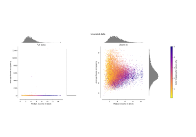
Compare the effect of different scalers on data with outliers