BP神经网络回归预测模型(python实现)
2018-03-20 17:35
791 查看
神经网络模型一般用来做分类,回归预测模型不常见,本文基于一个用来分类的BP神经网络,对它进行修改,实现了一个回归模型,用来做室内定位。模型主要变化是去掉了第三层的非线性转换,或者说把非线性激活函数Sigmoid换成f(x)=x函数。这样做的主要原因是Sigmoid函数的输出范围太小,在0-1之间,而回归模型的输出范围较大。模型修改如下:
 代码如下:#coding: utf8''''author: Huangyuliang'''import jsonimport randomimport sysimport numpy as np#### Define the quadratic and cross-entropy cost functionsclass CrossEntropyCost(object):@staticmethoddef fn(a, y):return np.sum(np.nan_to_num(-y*np.log(a)-(1-y)*np.log(1-a)))@staticmethoddef delta(z, a, y):return (a-y)#### Main Network classclass Network(object):def __init__(self, sizes, cost=CrossEntropyCost):self.num_layers = len(sizes)self.sizes = sizesself.default_weight_initializer()self.cost=costdef default_weight_initializer(self):self.biases = [np.random.randn(y, 1) for y in self.sizes[1:]]self.weights = [np.random.randn(y, x)/np.sqrt(x)for x, y in zip(self.sizes[:-1], self.sizes[1:])]def large_weight_initializer(self):self.biases = [np.random.randn(y, 1) for y in self.sizes[1:]]self.weights = [np.random.randn(y, x)for x, y in zip(self.sizes[:-1], self.sizes[1:])]def feedforward(self, a):"""Return the output of the network if ``a`` is input."""for b, w in zip(self.biases[:-1], self.weights[:-1]): # 前n-1层a = sigmoid(np.dot(w, a)+b)b = self.biases[-1] # 最后一层w = self.weights[-1]a = np.dot(w, a)+breturn adef SGD(self, training_data, epochs, mini_batch_size, eta,lmbda = 0.0,evaluation_data=None,monitor_evaluation_accuracy=False): # 用随机梯度下降算法进行训练n = len(training_data)for j in xrange(epochs):random.shuffle(training_data)mini_batches = [training_data[k:k+mini_batch_size] for k in xrange(0, n, mini_batch_size)]for mini_batch in mini_batches:self.update_mini_batch(mini_batch, eta, lmbda, len(training_data))print ("Epoch %s training complete" % j)if monitor_evaluation_accuracy:print ("Accuracy on evaluation data: {} / {}".format(self.accuracy(evaluation_data), j))def update_mini_batch(self, mini_batch, eta, lmbda, n):"""Update the network's weights and biases by applying gradientdescent using backpropagation to a single mini batch. The``mini_batch`` is a list of tuples ``(x, y)``, ``eta`` is thelearning rate, ``lmbda`` is the regularization parameter, and``n`` is the total size of the training data set."""nabla_b = [np.zeros(b.shape) for b in self.biases]nabla_w = [np.zeros(w.shape) for w in self.weights]for x, y in mini_batch:delta_nabla_b, delta_nabla_w = self.backprop(x, y)nabla_b = [nb+dnb for nb, dnb in zip(nabla_b, delta_nabla_b)]nabla_w = [nw+dnw for nw, dnw in zip(nabla_w, delta_nabla_w)]self.weights = [(1-eta*(lmbda/n))*w-(eta/len(mini_batch))*nwfor w, nw in zip(self.weights, nabla_w)]self.biases = [b-(eta/len(mini_batch))*nbfor b, nb in zip(self.biases, nabla_b)]def backprop(self, x, y):"""Return a tuple ``(nabla_b, nabla_w)`` representing thegradient for the cost function C_x. ``nabla_b`` and``nabla_w`` are layer-by-layer lists of numpy arrays, similarto ``self.biases`` and ``self.weights``."""nabla_b = [np.zeros(b.shape) for b in self.biases]nabla_w = [np.zeros(w.shape) for w in self.weights]# feedforwardactivation = xactivations = [x] # list to store all the activations, layer by layerzs = [] # list to store all the z vectors, layer by layerfor b, w in zip(self.biases[:-1], self.weights[:-1]): # 正向传播 前n-1层z = np.dot(w, activation)+bzs.append(z)activation = sigmoid(z)activations.append(activation)# 最后一层,不用非线性b = self.biases[-1]w = self.weights[-1]z = np.dot(w, activation)+bzs.append(z)activation = zactivations.append(activation)# backward pass 反向传播delta = (self.cost).delta(zs[-1], activations[-1], y) # 误差 Tj - Ojnabla_b[-1] = deltanabla_w[-1] = np.dot(delta, activations[-2].transpose()) # (Tj - Oj) * O(j-1)for l in xrange(2, self.num_layers):z = zs[-l] # w*a + bsp = sigmoid_prime(z) # z * (1-z)delta = np.dot(self.weights[-l+1].transpose(), delta) * sp # z*(1-z)*(Err*w) 隐藏层误差nabla_b[-l] = deltanabla_w[-l] = np.dot(delta, activations[-l-1].transpose()) # Errj * Oireturn (nabla_b, nabla_w)def accuracy(self, data):results = [(self.feedforward(x), y) for (x, y) in data]alist=[np.sqrt((x[0][0]-y[0])**2+(x[1][0]-y[1])**2) for (x,y) in results]return np.mean(alist)def save(self, filename):"""Save the neural network to the file ``filename``."""data = {"sizes": self.sizes,"weights": [w.tolist() for w in self.weights],"biases": [b.tolist() for b in self.biases],"cost": str(self.cost.__name__)}f = open(filename, "w")json.dump(data, f)f.close()#### Loading a Networkdef load(filename):"""Load a neural network from the file ``filename``. Returns aninstance of Network."""f = open(filename, "r")data = json.load(f)f.close()cost = getattr(sys.modules[__name__], data["cost"])net = Network(data["sizes"], cost=cost)net.weights = [np.array(w) for w in data["weights"]]net.biases = [np.array(b) for b in data["biases"]]return netdef sigmoid(z):"""The sigmoid function."""return 1.0/(1.0+np.exp(-z))def sigmoid_prime(z):"""Derivative of the sigmoid function."""return sigmoid(z)*(1-sigmoid(z))调用神经网络进行训练并保存参数:
 调用保存好的参数,进行定位预测:
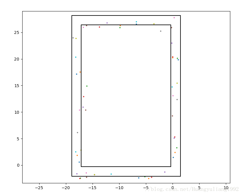 真实路径为行人从原点绕环形走廊一圈。
#coding: utf8
import my_datas_loader_1
import network_0

training_data,test_data = my_datas_loader_1.load_data_wrapper()
#### 训练网络,保存训练好的参数
net = network_0.Network([14,100,2],cost = network_0.CrossEntropyCost)
net.large_weight_initializer()
net.SGD(training_data,1000,316,0.005,lmbda =0.1,evaluation_data=test_data,monitor_evaluation_accuracy=True)
filename=r'C:\Users\hyl\Desktop\Second_158\Regression_Model\parameters.txt'
net.save(filename)
第190-199轮训练结果如下:
#coding: utf8
import my_datas_loader_1
import network_0
import matplotlib.pyplot as plt

test_data = my_datas_loader_1.load_test_data()
#### 调用训练好的网络,用来进行预测
filename=r'D:\Workspase\Nerual_networks\parameters.txt'      ## 文件保存训练好的参数
net = network_0.load(filename)                               ## 调用参数,形成网络
fig=plt.figure(1)
ax=fig.add_subplot(1,1,1)
ax.axis("equal")
# plt.grid(color='b' , linewidth='0.5' ,linestyle='-')        #  添加网格
x=[-0.3,-0.3,-17.1,-17.1,-0.3]                               ## 这是九楼地形的轮廓
y=[-0.3,26.4,26.4,-0.3,-0.3]
m=[1.5,1.5,-18.9,-18.9,1.5]
n=[-2.1,28.2,28.2,-2.1,-2.1]
ax.plot(x,y,m,n,c='k')

for i in range(len(test_data)):
pre = net.feedforward(test_data[i][0])  # pre 是预测出的坐标
bx=pre[0]
by=pre[1]
ax.scatter(bx,by,s=4,lw=2,marker='.',alpha=1)  #散点图
plt.pause(0.001)
plt.show()
定位精度达到了1.5米左右。定位效果如下图所示:
相关文章推荐
- 【Python学习系列二十四】scikit-learn库逻辑回归实现唯品会用户购买行为预测
- 机器学习经典算法详解及Python实现--CART分类决策树、回归树和模型树
- 常用统计学回归模型应用场景与python实现方法
- 机器学习实战(8) ——预测数值型数据回归(python实现)
- LSTM模型分析及对时序数据预测的具体实现(python实现)
- NN:实现BP神经网络的回归拟合,基于近红外光谱的汽油辛烷值含量预测结果对比—Jason niu
- 机器学习经典算法详解及Python实现--CART分类决策树、回归树和模型树
- python实现房价预测,采用回归和随机梯度下降法
- LSTM模型分析及对时序数据预测的具体实现(python实现)
- CART分类决策树、回归树和模型树算法详解及Python实现
- 神经网络实现连续型变量的回归预测(python)
- 简单数据预测—使用Python训练回归模型并进行预测(转自蓝鲸网站分析博客)
- 基于Scikit-learn实现回归模型——房价预测
- lda模型的python实现
- 【Python】scikit-learn机器学习(一)——一元回归模型
- python 实现 Peceptron Learning Algorithm ( 二) 感知机模型实现
- python 实现 Peceptron Learning Algorithm ( 三) 感知机模型应用于Iris数据集
- Python实现LR(逻辑回归)
- Logistic回归 Python实现
- 机器学习实战笔记(Python实现)-08-线性回归