Windows10 GPU版Tensorflow配置教程+Anaconda3+Jupyter Notebook

pip

pip install 你要装的包 -i https://pypi.tuna.tsinghua.edu.cn/simple[/code] 
二、正式开始

先安利两个网站

Tensorflow官方安装教程

Tensorflow中文社区

第一个可能要fan墙。

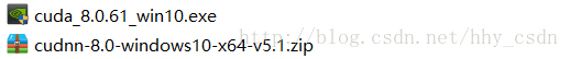
首先下载CUDA和cuDNN

CUDA的所有历史版本

我用的是CUDA8.0，用起来没问题，最新版9.1没试过。

cuDNN5.1对应CUDA8.0



先安装第一个EXE文件，按照安装程序走下来就可以。第二个压缩包，将解压出来的三个文件夹覆盖到第一个的安装目录下。



然后下载Anaconda3

Anaconda的威力不用再多说了，集成了很多package，也有多版本的python管理，用起来很是方便。

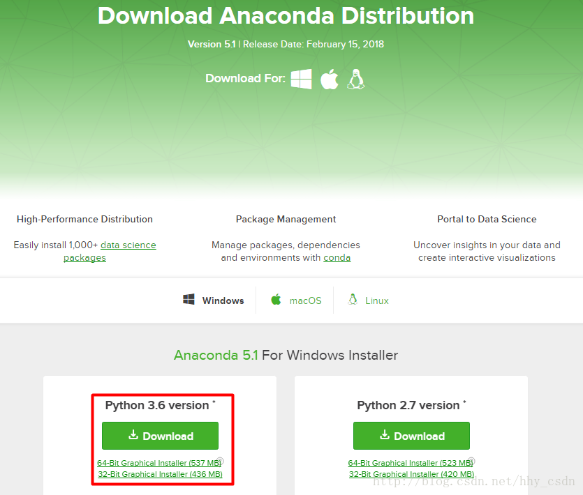
首先上官网Anaconda官网



因为Windows环境下的
Tensorflow
支持
Python3.5
或是
Python3.6
，所以要下载红框里的版本。如果想安装与
Python3.5
相匹配的
Anaconda3
，有两个办法：

在这个网站下载Anaconda3-4.2.0-Windows-x86_64.exe然后安装即可。

下载最新版的Anaconda3，然后用python版本管理功能新建一个
Python3.5
环境即可。下面的步骤会详细讲这个如何操作。

强烈建议大家下载Anaconda3 4.2.0版本，最新版我又试了一下，自带的python总是3.6版本，装了几次Tensorflow都不成功，最后卸了最新版Anaconda，装回4.2.0，回到了熟悉的python3.5.2就没有问题了
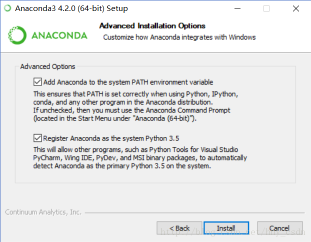
在这个网站下载Anaconda3-4.2.0-Windows-x86_64.exe然后安装

Anaconda3的安装截图



按照默认安装即可。

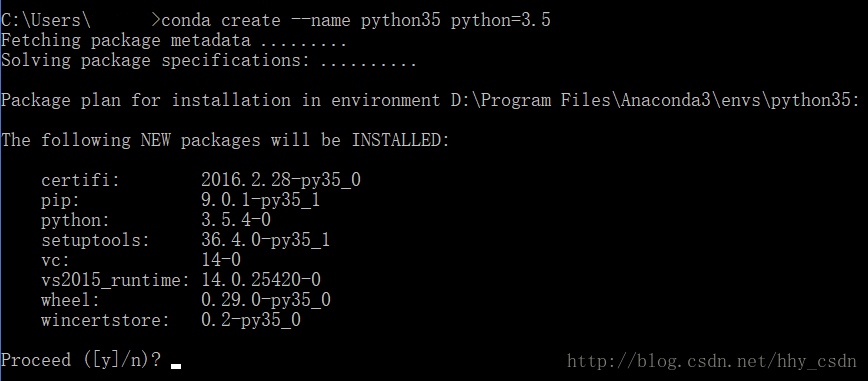
下面我们利用
conda
命令建立一个
Pyhton3.5
的环境，当然，如果有其他需要，也可以建立一个
Pyhton2.7
 
Python3.6
等等不同的版本环境，不同的环境之间互不干扰。

打开命令行cmd，建议用管理员模式。

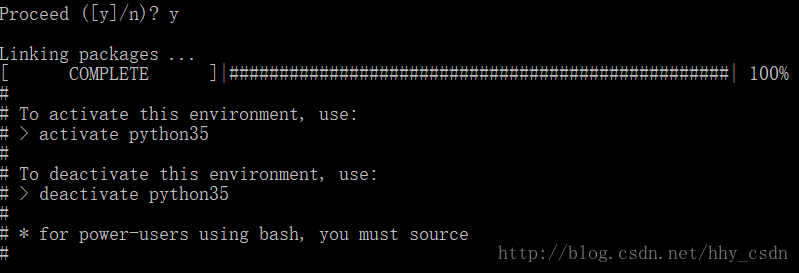
输入
conda create --name python35 python=3.5
输入y，稍等片刻即可建立一个新环境。如果在建立的这个环境里不成功的话，尝试建立
conda create --name Anaconda3
，再走一遍下面的操作。

还是建议大家使用
conda create --name Anaconda3
，并且检查一下python版本是不是3.5.2，虽说win版tf支持3.6但是毕竟3.5.2还是最稳定的。




3. 用
activate python35
或者
activate Anaconda3
激活刚刚配置好的环境。需要退出该环境时，用
deactivate python35
或
deactivate Anaconda3




C盘符前面的
（Anaconda3）
说明进入了该环境。

4. 运行
python
确认3.5版本无误，
ctrl+Z
退出
python


5. 运行
jupyter notebook
,浏览器自动弹出Jupyter Notebook界面，无误。

6. 回到
conda
环境，输入

pip install tensorflow-gpu==1.2.0 -i https://pypi.tuna.tsinghua.edu.cn/simple[/code] 
安装1.2.0版本的tensorflow，主要是如果不加
==1.2.0
默认安装的是最新的tensorflow，1.6.0版本，和CUDA8.0不匹配，导致jupyter notebook下无法成功
import tensorflow
，爆出这个错误

1.OSError: [WinError 126] 找不到指定的模块。
2.ImportError: Could not find 'cudart64_90.dll'. TensorFlowrequires that this DLL be installed in a directory that is     named in your %PATH%environment variable. Download and install CUDA 9.0 from this URL:  https://developer.nvidia.com/cuda-toolkit


如果安装不出问题的话，到此安装过程就顺利结束了。

下面测试一下。

在conda环境下进入python，

import tensorflow as tf
#查看版本号
tf.__version__
#查看安装路径
tf.__path__


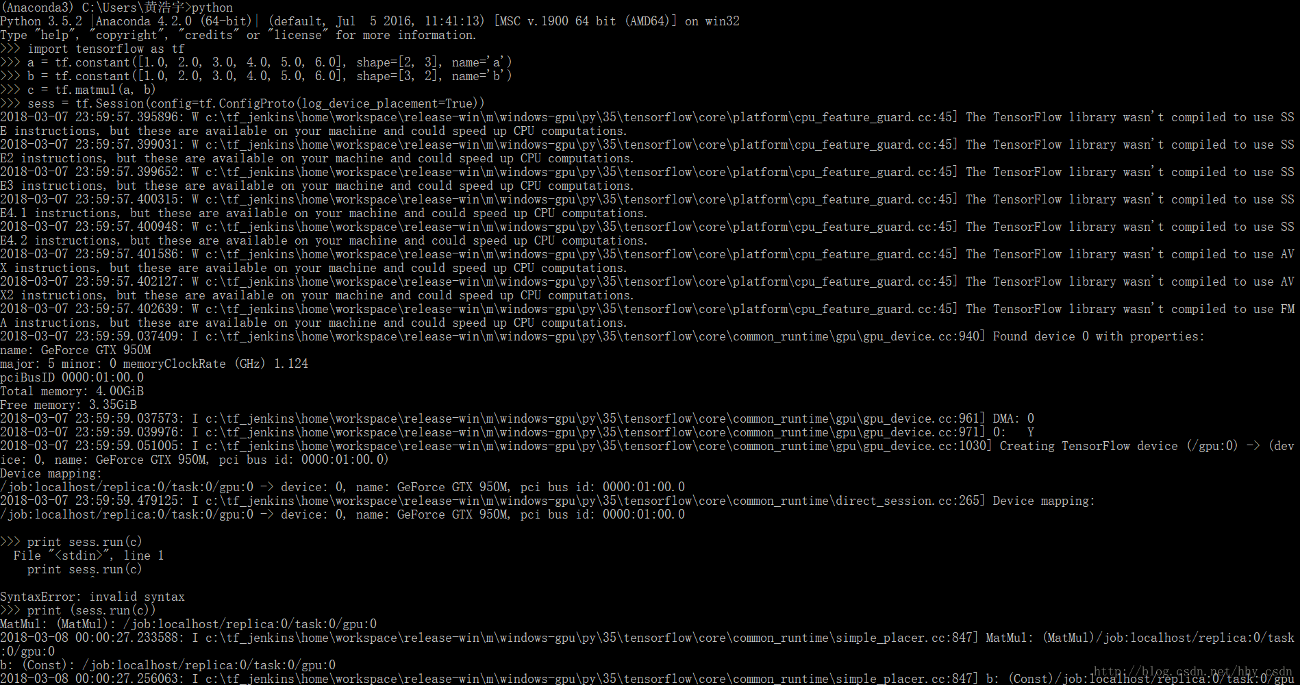
输入官方教程代码

#Creates a graph.
a = tf.constant([1.0, 2.0, 3.0, 4.0, 5.0, 6.0], shape=[2, 3], name='a')
b = tf.constant([1.0, 2.0, 3.0, 4.0, 5.0, 6.0], shape=[3, 2], name='b')
c = tf.matmul(a, b)
#Creates a session with log_device_placement set to True.
sess = tf.Session(config=tf.ConfigProto(log_device_placement=True))
#Runs the op.
print (sess.run(c))


输出





可见tensorflow在计算时成功调用了GPU，并且输出正确。

在
jupyter notebook
下测试。

我用的是logistic 回归的一段训练代码

import tensorflow as tf
x_data = [[1, 2], [2, 3], [3, 1], [4, 3], [5, 3], [6, 2]]
y_data = [[0], [0], [0], [1], [1], [1]]
# pl
b4e1
aceholders for a tensor that will be always fed.
X = tf.placeholder(tf.float32, shape=[None, 2])
Y = tf.placeholder(tf.float32, shape=[None, 1])

W = tf.Variable(tf.random_normal([2, 1]), name='weight')
b = tf.Variable(tf.random_normal([1]), name='bias')
# Hypothesis using sigmoid: tf.div(1., 1. + tf.exp(tf.matmul(X, W)))
hypothesis = tf.sigmoid(tf.matmul(X, W) + b)
# cost/loss function
cost = -tf.reduce_mean(Y * tf.log(hypothesis) + (1 - Y) * tf.log(1 - hypothesis))
train = tf.train.GradientDescentOptimizer(learning_rate=0.01).minimize(cost)

# Accuracy computation
# True if hypothesis>0.5 else False
predicted = tf.cast(hypothesis > 0.5, dtype=tf.float32)
accuracy = tf.reduce_mean(tf.cast(tf.equal(predicted, Y), dtype=tf.float32))

# Launch graph
with tf.Session() as sess:
# Initialize TensorFlow variables
sess.run(tf.global_variables_initializer())

for step in range(10001):
cost_val, _ = sess.run([cost, train], feed_dict={X: x_data, Y: y_data})
if step % 200 == 0:
print(step, cost_val)

# Accuracy report
h, c, a = sess.run([hypothesis, predicted, accuracy],
feed_dict={X: x_data, Y: y_data})
print("\nHypothesis: ", h, "\nCorrect (Y): ", c, "\nAccuracy: ", a)


输出日志

0 1.4967082
200 0.7839919
400 0.53214276
600 0.43306607
800 0.3880737
1000 0.36270094
1200 0.34548092
1400 0.33213395
1600 0.3208673
1800 0.3108564
2000 0.3016926
2200 0.2931581
2400 0.28512952
2600 0.27753118
2800 0.27031356
3000 0.26344112
3200 0.25688663
3400 0.25062782
3600 0.24464555
3800 0.23892312
4000 0.23344503
4200 0.22819762
4400 0.22316761
4600 0.2183432
4800 0.21371302
5000 0.20926651
5200 0.20499402
5400 0.20088613
5600 0.19693428
5800 0.19313025
6000 0.18946663
6200 0.1859361
6400 0.182532
6600 0.17924798
6800 0.1760783
7000 0.17301725
7200 0.17005971
7400 0.16720062
7600 0.16443534
7800 0.16175961
8000 0.15916926
8200 0.15666038
8400 0.15422934
8600 0.15187272
8800 0.14958727
9000 0.14736985
9200 0.14521751
9400 0.1431275
9600 0.14109737
9800 0.13912444
10000 0.13720647

Hypothesis:  [[0.02574597]
[0.15147369]
[0.27998957]
[0.7929884 ]
[0.946652  ]
[0.98256886]]
Correct (Y):  [[0.]
[0.]
[0.]
[1.]
[1.]
[1.]]
Accuracy:  1.0


结果完美，大功告成！

PS：最后可以安装一下Keras，
pip install keras –i https://pypi.tuna.tsinghua.edu.cn/simple[/code]