图的DFS和BFS算法解析
2018-03-07 16:04
302 查看
图是一种灵活的数据结构,一般作为一种模型用来定义对象之间的关系或联系。对象由
在图的基本算法中,最初需要接触的就是图的遍历算法,根据访问节点的顺序,可分为广度优先搜索(BFS)和深度优先搜索(DFS)。
本文将给出给出BFS和DFS的以下几种实现方式:
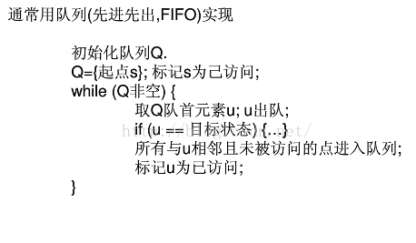
1、使用队列Queue实现图的BFS遍历
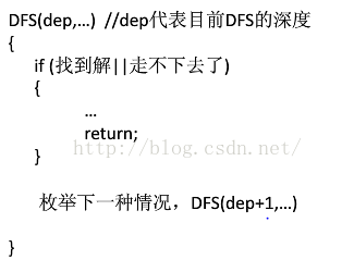
2、递归实现图的DFS遍历
3、使用栈Stack迭代实现图的DFS遍历
同深度优先搜索相反,BFS宽度优先搜索每次选择深度最浅的节点优先扩展。并且当问题有解时,宽度优先算法一定能够找到解,并且在单位耗散时间的情况下,可以保证找到最优解。
对于深度优先搜索算法的思想。在一般情况下,当问题有解时,深度优先搜索不但不能够保证找到最优解,也不能保证找到解。如果问题状态空间有限,则可以保证找到解;但是当问题的状态空间无限时,则可能陷入“深渊”而找不到解。为此我们可以利用
使用栈实现DFS思路关键点:
1、首先明确整个DFS主要便是对于栈进行操作,就是在顶点压栈和弹栈过程中我们需要进行的操作;
2、利用DFS的思想,深度遍历节点。直到栈内元素为空位置;
3、何时进行压栈:对于栈顶顶点,看其邻接顶点中是够存在未被遍历过得白色顶点,若有则对将其压栈,然后再对栈顶元素进行操作;
4、如果栈顶顶点的所有邻接顶点都是被遍历过的灰色顶点,则将栈顶元素弹栈,然后再对现在的栈顶元素进行操作;
5、算法结束时,所有元素均被遍历过即为灰色,并且栈已经为空。
DFS适合此类题目:给定初始状态跟目标状态,要求判断从初始状态到目标状态是否有解
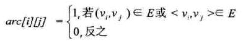
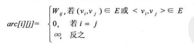
设图G有n个顶点,则邻接矩阵是一个n*n的方阵,定义为:
无向图:
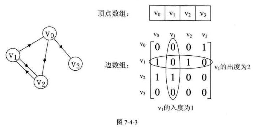
有向图:
在图的术语中,我们提到了
设图G是网图,有n个顶点,则邻接矩阵是一个n*n的方阵,定义为:
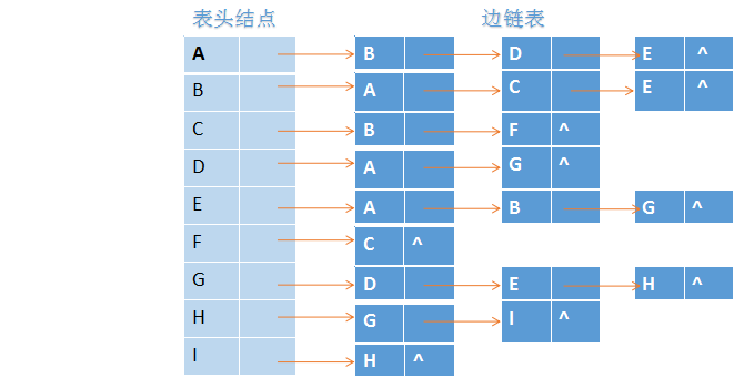
所有表头结点以顺序结构的形式存储,以便可以随机访问任一顶点的边链表。上图的邻接链表表示法如下:
顶点(V)表示,而对象之间的关系或者关联则通过图的
边(E)来表示。
在图的基本算法中,最初需要接触的就是图的遍历算法,根据访问节点的顺序,可分为广度优先搜索(BFS)和深度优先搜索(DFS)。
本文将给出给出BFS和DFS的以下几种实现方式:
1、使用队列Queue实现图的BFS遍历
2、递归实现图的DFS遍历
3、使用栈Stack迭代实现图的DFS遍历
一、BFS(广度优先搜索算法)
BFS算法之所以叫做广度优先搜索,是因为它始终将已发现的顶点和未发现的之间的边界,沿其广度方向向外扩展。亦即,算法首先会发现和s距离为k的所有顶点,然后才会发现和s距离为k+1的其他顶点。同深度优先搜索相反,BFS宽度优先搜索每次选择深度最浅的节点优先扩展。并且当问题有解时,宽度优先算法一定能够找到解,并且在单位耗散时间的情况下,可以保证找到最优解。
Java代码实现:
class Node1 {
int x;
Node1 next;
public Node1(int x) {
this.x = x;
this.next = null;
}
}
public class BFS {
public Node1 first;
public Node1 last;

public static int run[] = new int[9];
public static BFS head[] = new BFS[9];
public final static int MAXSIZE = 10;
static int[] queue = new int[MAXSIZE];
static int front = -1;
static int rear = -1;

public static void enqueue(int value) {
if(rear>=MAXSIZE) return;
rear++;
queue[rear] = value;
}

public static int dequeue() {
if(front == rear) return -1;
front++;
return queue[front];
}

public static void bfs(int current) {
Node1 tempNode1;
enqueue(current);
run[current] = 1;
System.out.print("[" + current + "]");
while (front != rear) {
current = dequeue();
tempNode1 = head[current].first;
while (tempNode1 != null) {
if(run[tempNode1.x] == 0) {
enqueue(tempNode1.x);
run[tempNode1.x] = 1;
System.out.print("[" + tempNode1.x + "]");
}
tempNode1 = tempNode1.next;
}
}
}

public boolean isEmpty() {
return first == null;
}

public void print() {
Node1 current = first;
while(current != null) {
System.out.print("[" + current.x + "]");
current = current.next;
}
System.out.println();
}
public void insert(int x) {
Node1 newNode1 = new Node1(x);
if(this.isEmpty()) {
first = newNode1;
last = newNode1;
}
else {
last.next = newNode1;
last = newNode1;
}
}

public static void main(String[] args) {
int Data[][] = { {1,2}, {2,1}, {1,3}, {3,1}, {2,4}, {4,2},
{2,5}, {5,2}, {3,6}, {6,3}, {3,7}, {7,3}, {4,5}, {5,4},
{6,7}, {7,6}, {5,8}, {8,5}, {6,8}, {8,6} };
int DataNum;
int i,j;
System.out.println("图形的邻接表内容为:");
for(i=1;i<9;i++) {
run[i] = 0;
head[i] = new BFS();
System.out.print("顶点" + i + "=>");
for (j=0;j<20;j++) {
if(Data[j][0] == i) {
DataNum = Data[j][1];
head[i].insert(DataNum);
}
}
head[i].print();
}
System.out.println("深度优先遍历顶点:");
bfs(1);
System.out.println("");
}

}
二、DFS(深度优先搜索算法)
DFS算法利用递归方式实现,和BFS不同的是BFS搜索产生的始终是一棵树,而DFS产生的可能会使一个森林。
对于深度优先搜索算法的思想。在一般情况下,当问题有解时,深度优先搜索不但不能够保证找到最优解,也不能保证找到解。如果问题状态空间有限,则可以保证找到解;但是当问题的状态空间无限时,则可能陷入“深渊”而找不到解。为此我们可以利用
回溯算法中的思想,可以加上对搜索的深度限制。从而实现对于搜索深度的限制。当然深度限制设置必须合理,深度过深则影响搜索的效率,深度过浅时,则可能影响找到问题的解。
使用栈实现DFS思路关键点:
1、首先明确整个DFS主要便是对于栈进行操作,就是在顶点压栈和弹栈过程中我们需要进行的操作;
2、利用DFS的思想,深度遍历节点。直到栈内元素为空位置;
3、何时进行压栈:对于栈顶顶点,看其邻接顶点中是够存在未被遍历过得白色顶点,若有则对将其压栈,然后再对栈顶元素进行操作;
4、如果栈顶顶点的所有邻接顶点都是被遍历过的灰色顶点,则将栈顶元素弹栈,然后再对现在的栈顶元素进行操作;
5、算法结束时,所有元素均被遍历过即为灰色,并且栈已经为空。
DFS的思想是从一个顶点V0开始,沿着一条路一直走到底,如果发现不能到达目标解,那就返回到上一个节点,然后从另一条路开始走到底。
DFS适合此类题目:给定初始状态跟目标状态,要求判断从初始状态到目标状态是否有解
Java代码实现:
class Node {
int x;
Node next;
public Node(int x) {
this.x = x;
this.next = null;
}
}
public class DFS {
public Node first;
public Node last;

public static int run[] = new int[9];
public static DFS head[] = new DFS[9];

public static void dfs(int current) {
run[current] = 1;
System.out.print("[" + current + "]");

while (head[current].first != null) {
if (run[head[current].first.x] == 0) { //如果顶点尚未遍历,就进行dfs递归
dfs(head[current].first.x);
}
head[current].first = head[current].first.next;
}
}

public boolean isEmpty() {
return first == null;
}

public void print() {
Node current = first;
while (current != null) {
System.out.print("[" + current.x + "]");
current = current.next;
}
System.out.println();
}

public void insert(int x) {
Node newNode = new Node(x);
if (this.isEmpty()) {
first = newNode;
last = newNode;
} else {
last.next = newNode;
last = newNode;
}
}

public static void main(String[] args) {
int Data[][] = {{1, 2}, {2, 1}, {1, 3}, {3, 1}, {2, 4}, {4, 2},
{2, 5}, {5, 2}, {3, 6}, {6, 3}, {3, 7}, {7, 3}, {4, 5}, {5, 4},
{6, 7}, {7, 6}, {5, 8}, {8, 5}, {6, 8}, {8, 6}};
int DataNum;
int i, j;
System.out.println("图形的邻接表内容为:");
for (i = 1; i < 9; i++) {
run[i] = 0;
head[i] = new DFS();
System.out.print("顶点" + i + "=>");
for (j = 0; j < 20; j++) {
if (Data[j][0] == i) {
DataNum = Data[j][1];
head[i].insert(DataNum);
}
}
head[i].print();
}
System.out.println("深度优先遍历顶点:");
dfs(1);
System.out.println("");
}
}
图的两种存储方式:
要存储一个图,我们知道图既有结点,又有边,对于有权图来说,每条边上还带有权值。常用的图的存储结构主要有以下二种:1.邻接矩阵
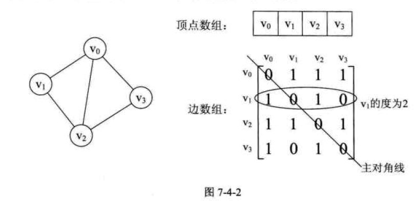
图的邻接矩阵(Adjacency Matrix)存储方式是用两个数组来表示图。一个一维的数组存储图中顶点信息,一个二维数组(称为邻接矩阵)存储图中的边或弧的信息。设图G有n个顶点,则邻接矩阵是一个n*n的方阵,定义为:
无向图:
解释:若Vi和Vj之间有连接为1,没有连接为0
有向图:
在图的术语中,我们提到了
网的概念,也就是每条边上都带有权的图叫做网。那些这些权值就需要保存下来。
设图G是网图,有n个顶点,则邻接矩阵是一个n*n的方阵,定义为:
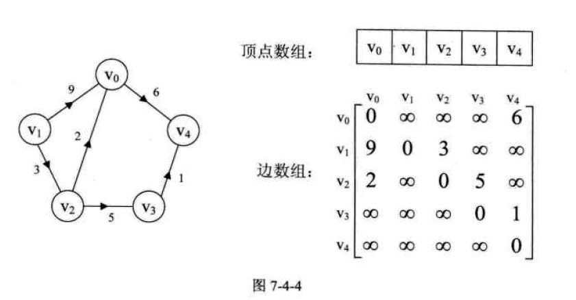
2.邻接表
邻接链表表示法对图中的每个顶点建立一个带头的边链表;第i条链表代表依附于顶点vivi所有边信息,若为有向图,则表示以顶点vivi为弧尾的边信息。邻接链接可以分为两部分,表头结点定义了顶点信息,随后的边链表表达了关于此顶点边信息。所有表头结点以顺序结构的形式存储,以便可以随机访问任一顶点的边链表。上图的邻接链表表示法如下:
