关于MatConvNet的反向传播原理及源码解析

MatConvNet深度学习库的反向传播原理如下图所示：



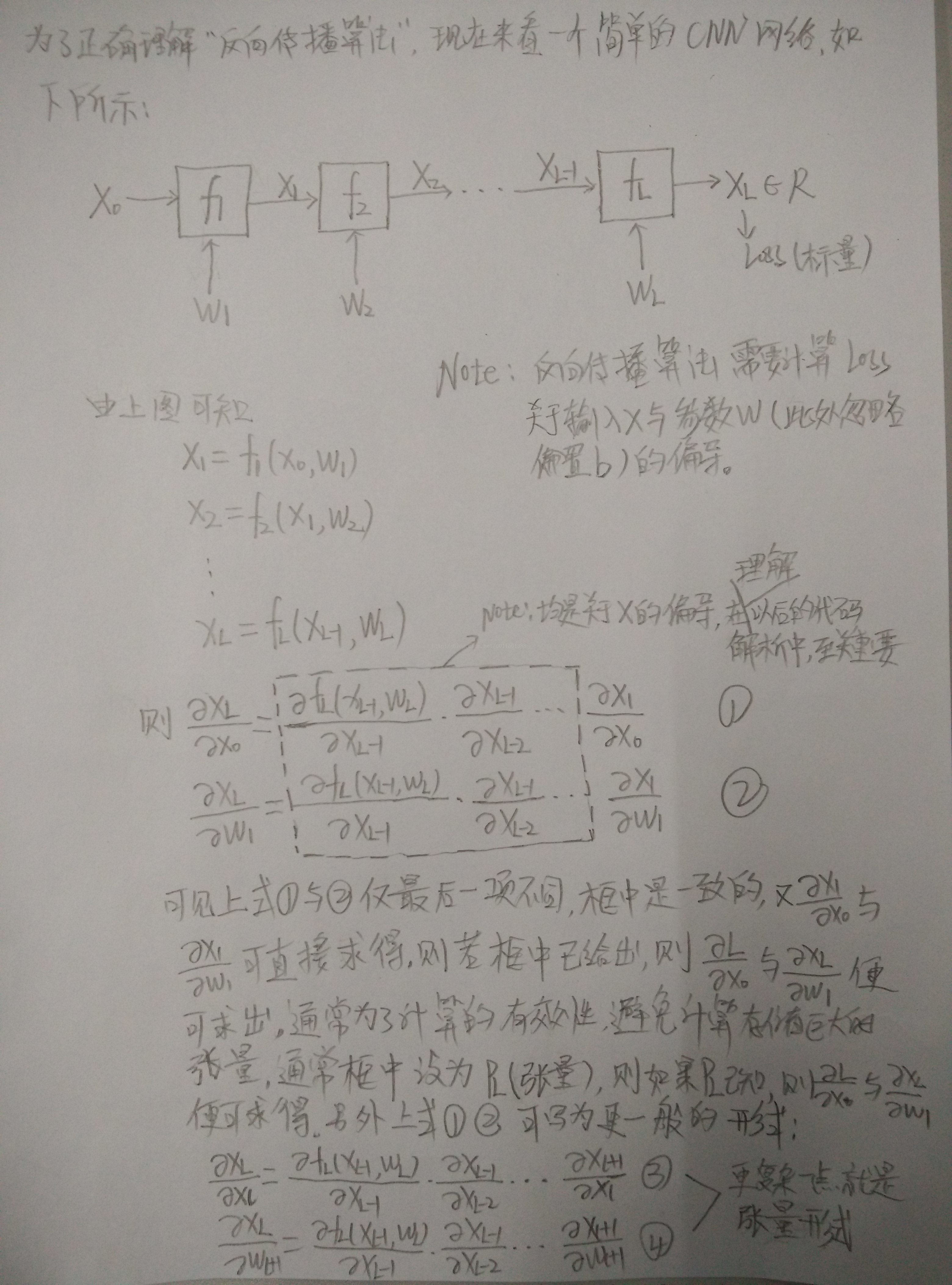
上图是简化版的反向传播原理推导，具体的张量表示法参考相关手册。

为了方便对比及具体详尽的原理推导，在手册中，关于反向传播的推导部分截图如下：





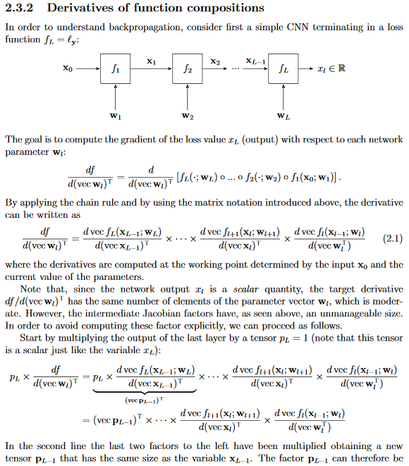
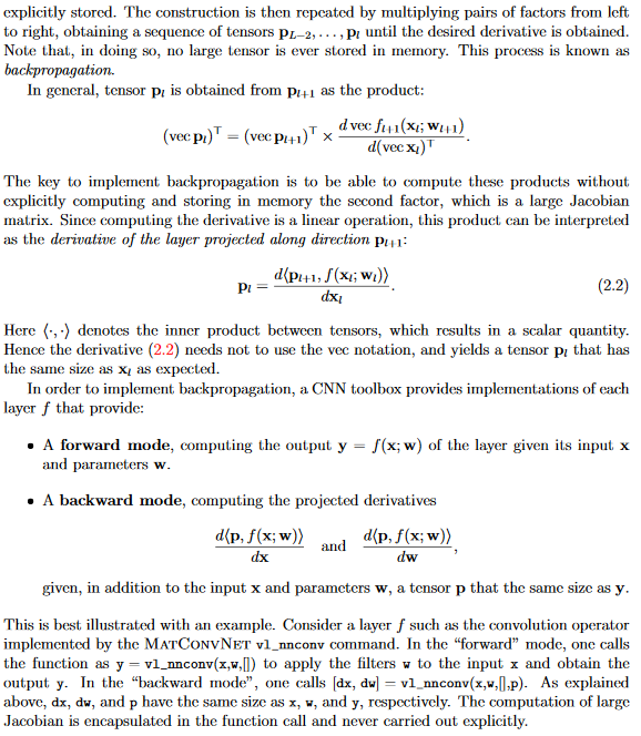
其中在上图中，重点注意的地方就是式（2.2），它只是关于x的导数。为了引起重视，下面有一个练习：

%下面实现一个由一个卷积层和ReLU层构成的两层卷积网络的反向传播实现示例

%前向模式：计算卷积和卷积后的ReLU输出
y = vl_nnconv(x, w, []) ;
z = vl_nnrelu(y) ;

%初始化一个随机投影张量
p = randn(size(z), 'single') ;

%反向传播模式：映射偏导
dy = vl_nnrelu(z, p) ;
[dx,dw] = vl_nnconv(x, w, [], dy) ;
那么，修改上述代码，实现一个级联的Conv+ReLU+Conv网络，该如何实现呢？尤其是在反向模式下，vl_nnconv的第四个参数偏导该传入什么呢？会在后面给出完整参考代码。
下面进行反向传播的MatConvNet的反向传播实现方式：

res = struct(...
'x', cell(1,n+1), ...
'dzdx', cell(1,n+1), ...
'dzdw', cell(1,n+1), ...
'aux', cell(1,n+1), ...
'stats', cell(1,n+1), ...
'time', num2cell(zeros(1,n+1)), ...
'backwardTime', num2cell(zeros(1,n+1))) ;

% -------------------------------------------------------------------------
% Backward pass
% -------------------------------------------------------------------------

if doder
res(n+1).dzdx = dzdy ;
for i=n:-1:backPropLim
l = net.layers{i} ;
res(i).backwardTime = tic ;
switch l.type

case 'conv'
[res(i).dzdx, dzdw{1}, dzdw{2}] = ...
vl_nnconv(res(i).x, l.weights{1}, l.weights{2}, res(i+1).dzdx, ...
'pad', l.pad, ...
'stride', l.stride, ...
'dilate', l.dilate, ...
l.opts{:}, ...
cudnn{:}) ;

case 'convt'
[res(i).dzdx, dzdw{1}, dzdw{2}] = ...
vl_nnconvt(res(i).x, l.weights{1}, l.weights{2}, res(i+1).dzdx, ...
'crop', l.crop, ...
'upsample', l.upsample, ...
'numGroups', l.numGroups, ...
l.opts{:}, ...
cudnn{:}) ;

case 'pool'
res(i).dzdx = vl_nnpool(res(i).x, l.pool, res(i+1).dzdx, ...
'pad', l.pad, 'stride', l.stride, ...
'method', l.method, ...
l.opts{:}, ...
cudnn{:}) ;

case {'normalize', 'lrn'}
res(i).dzdx = vl_nnnormalize(res(i).x, l.param, res(i+1).dzdx) ;

case 'softmax'
res(i).dzdx = vl_nnsoftmax(res(i).x, res(i+1).dzdx) ;

case 'loss'
res(i).dzdx = vl_nnloss(res(i).x, l.class, res(i+1).dzdx) ;

case 'softmaxloss'
res(i).dzdx = vl_nnsoftmaxloss(res(i).x, l.class, res(i+1).dzdx) ;

case 'relu'
if l.leak > 0, leak = {'leak', l.leak} ; else leak = {} ; end
if ~isempty(res(i).x)
res(i).dzdx = vl_nnrelu(res(i).x, res(i+1).dzdx, leak{:}) ;
else
% if res(i).x is empty, it has been optimized away, so we use this
% hack (which works only for ReLU):
res(i).dzdx = vl_nnrelu(res(i+1).x, res(i+1).dzdx, leak{:}) ;
end

case 'sigmoid'
res(i).dzdx = vl_nnsigmoid(res(i).x, res(i+1).dzdx) ;

case 'noffset'
res(i).dzdx = vl_nnnoffset(res(i).x, l.param, res(i+1).dzdx) ;

case 'spnorm'
res(i).dzdx = vl_nnspnorm(res(i).x, l.param, res(i+1).dzdx) ;

case 'dropout'
if testMode
res(i).dzdx = res(i+1).dzdx ;
else
res(i).dzdx = vl_nndropout(res(i).x, res(i+1).dzdx, ...
'mask', res(i+1).aux) ;
end

case 'bnorm'
[res(i).dzdx, dzdw{1}, dzdw{2}, dzdw{3}] = ...
vl_nnbnorm(res(i).x, l.weights{1}, l.weights{2}, res(i+1).dzdx, ...
'epsilon', l.epsilon, ...
bnormCudnn{:}) ;
% multiply the moments update by the number of images in the batch
% this is required to make the update additive for subbatches
% and will eventually be normalized away
dzdw{3} = dzdw{3} * size(res(i).x,4) ;

case 'pdist'
res(i).dzdx = vl_nnpdist(res(i).x, l.class, ...
l.p, res(i+1).dzdx, ...
'noRoot', l.noRoot, ...
'epsilon', l.epsilon, ...
'aggregate', l.aggregate, ...
'instanceWeights', l.instanceWeights) ;

case 'custom'
res(i) = l.backward(l, res(i), res(i+1)) ;

end % layers

switch l.type
case {'conv', 'convt', 'bnorm'}
if ~opts.accumulate
res(i).dzdw = dzdw ;
else
for j=1:numel(dzdw)
res(i).dzdw{j} = res(i).dzdw{j} + dzdw{j} ;
end
end
dzdw = [] ;
if ~isempty(opts.parameterServer) && ~opts.holdOn
for j = 1:numel(res(i).dzdw)
opts.parameterServer.push(sprintf('l%d_%d',i,j),res(i).dzdw{j}) ;
res(i).dzdw{j} = [] ;
end
end
end
if opts.conserveMemory && ~net.layers{i}.precious && i ~= n
res(i+1).dzdx = [] ;
res(i+1).x = [] ;
end
if gpuMode && opts.sync
wait(gpuDevice) ;
end
res(i).backwardTime = toc(res(i).backwardTime) ;
end
if i > 1 && i == backPropLim && opts.conserveMemory && ~net.layers{i}.precious
res(i).dzdx = [] ;
res(i).x = [] ;
end
end

由上述实现方式，练习题的参考答案如下：
%下面实现一个由Conv+ReLU+Conv构成的三层卷积网络的反向传播实现示例

%前向模式：计算卷积和卷积后的ReLU输出
y = vl_nnconv(x, w, []) ;
z = vl_nnrelu(y) ;
y1=vl_nnconv(z,w,[]);

%初始化一个随机投影张量
p = randn(size(y1), 'single') ;

%反向传播模式：映射偏导
[dz,dw]=vl_nnconv(z,w,[],p);
dy = vl_nnrelu(y, dz) ;
[dx,dw] = vl_nnconv(x, w, [], dy) ;