TersorflowTutorial_MNIST数据集上简单CNN实现
2018-02-11 20:55
726 查看
MNIST数据集上简单CNN实现
觉得有用的话,欢迎一起讨论相互学习~Follow Me
参考文献Tensorflow机器学习实战指南
源代码请点击下方链接欢迎加星
Tesorflow实现基于MNIST数据集上简单CNN少说废话多写代码
下载并读取MNIST数据集
import matplotlib.pyplot as plt
import numpy as np
import tensorflow as tf
from tensorflow.contrib.learn.python.learn.datasets.mnist import read_data_sets
from tensorflow.python.framework import ops

ops.reset_default_graph()

# Start a graph session
sess = tf.Session()

# 下载并读取数据集
# 如果本地没有temp文件夹需要从Tensorflow官网下载
data_dir = 'temp'
mnist = read_data_sets(data_dir)

# 把mnist.train.images中的数据集变换成(28*28)的数据格式,原文件中以784维向量的形式保存
train_xdata = np.array([np.reshape(x, (28, 28)) for x in mnist.train.images])
test_xdata = np.array([np.reshape(x, (28, 28)) for x in mnist.test.images])
# print(train_xdata.shape)  # 输出格式是numpy.ndarray的形式
# print(test_xdata.shape)
# (55000, 28, 28)
# (10000, 28, 28)

train_labels = mnist.train.labels
test_labels = mnist.test.labels
# print(train_labels.shape)  # (55000,)
# print(train_labels[0:10])  # [7 3 4 6 1 8 1 0 9 8]
构造模型
# 设置模型超参数
batch_size = 100  # 批处理数量
learning_rate = 0.005  # 学习率
evaluation_size = 500  # 测试批数量
image_width = train_xdata[0].shape[0]
image_height = train_xdata[0].shape[1]
target_size = max(train_labels) + 1
# print(target_size)  # 10
num_channels = 1  # 通道数,灰度图片只有一个通道
generations = 500  # 迭代次数为500次
eval_every = 5  # 输出统计
conv1_features = 25  # 第一个卷积层特征个数
conv2_features = 50  # 第二个卷积层特征个数
max_pool_size1 = 2  # NxN window for 1st max pool layer
max_pool_size2 = 2  # NxN window for 2nd max pool layer
fully_connected_size1 = 100  # 全连接层神经元个数

# 声明模型占位符
# 训练数据集变量
x_input_shape = (batch_size, image_width, image_height, num_channels)
x_input = tf.placeholder(tf.float32, shape=x_input_shape)
y_target = tf.placeholder(tf.int32, shape=(batch_size))
# 测试数据集变量
eval_input_shape = (evaluation_size, image_width, image_height, num_channels)
eval_input = tf.placeholder(tf.float32, shape=eval_input_shape)
eval_target = tf.placeholder(tf.int32, shape=(evaluation_size))

# conv1_weight表示第一层的权重,即为第一层的卷积核[卷积核高,卷积核宽,输入通道数量,输出通道数量]
# 使用标准差为0.1的截断高斯分布进行变量初始化。注意通tf.Variable,此时的conv1_weight是一个变量。
conv1_weight = tf.Variable(tf.truncated_normal([4, 4, num_channels, conv1_features],
stddev=0.1, dtype=tf.float32))
# 第一个卷积层偏置
conv1_bias = tf.Variable(tf.zeros([conv1_features], dtype=tf.float32))

# 第二个卷积层权重即卷积核大小
conv2_weight = tf.Variable(tf.truncated_normal([4, 4, conv1_features, conv2_features],

stddev=0.1, dtype=tf.float32))
# 第二个卷积层偏置
conv2_bias = tf.Variable(tf.zeros([conv2_features], dtype=tf.float32))

# 全连接层参数
# 因为卷积层设置padding mode 为'SAME',所以卷积过后每一个特征层的维度仍与原来保持相同
# 在池化层中步长和窗口的宽度和高度相同,则进行池化操作后的输出的高度和宽度只是原维度除以池化窗口的乘积
resulting_width = image_width//(max_pool_size1*max_pool_size2)  # // 表示取整除法
resulting_height = image_height//(max_pool_size1*max_pool_size2)
full1_input_size = resulting_width*resulting_height*conv2_features
full1_weight = tf.Variable(tf.truncated_normal([full1_input_size, fully_connected_size1],
stddev=0.1, dtype=tf.float32))
full1_bias = tf.Variable(tf.truncated_normal([fully_connected_size1], stddev=0.1, dtype=tf.float32))
full2_weight = tf.Variable(tf.truncated_normal([fully_connected_size1, target_size],
stddev=0.1, dtype=tf.float32))
full2_bias = tf.Variable(tf.truncated_normal([target_size], stddev=0.1, dtype=tf.float32))

# 模型进行初始化操作
def my_conv_net(input_data):
# 第一个卷积-ReLU-池化层
conv1 = tf.nn.conv2d(input_data, conv1_weight, strides=[1, 1, 1, 1], padding='SAME')
relu1 = tf.nn.relu(tf.nn.bias_add(conv1, conv1_bias))
max_pool1 = tf.nn.max_pool(relu1, ksize=[1, max_pool_size1, max_pool_size1, 1],
strides=[1, max_pool_size1, max_pool_size1, 1], padding='SAME')
# 第二个卷积-ReLU-池化层
conv2 = tf.nn.conv2d(max_pool1, conv2_weight, strides=[1, 1, 1, 1], padding='SAME')
relu2 = tf.nn.relu(tf.nn.bias_add(conv2, conv2_bias))
max_pool2 = tf.nn.max_pool(relu2, ksize=[1, max_pool_size2, max_pool_size2, 1],
strides=[1, max_pool_size2, max_pool_size2, 1], padding='SAME')

# 扁平化/光栅化处理
# 将max_pool2的输出形状转化成list格式,其中分别表示[batch_size,height,weight,channels]
final_conv_shape = max_pool2.get_shape().as_list()
final_shape = final_conv_shape[1]*final_conv_shape[2]*final_conv_shape[3]
flat_output = tf.reshape(max_pool2, [final_conv_shape[0], final_shape])

# 第一个全连接层
fully_connected1 = tf.nn.relu(tf.add(tf.matmul(flat_output, full1_weight), full1_bias))

# 第二个全连接层
final_model_output = tf.add(tf.matmul(fully_connected1, full2_weight), full2_bias)

return (final_model_output)

# 构造好模型后,使用时只需要传入数据集
model_output = my_conv_net(x_input)
test_model_output = my_conv_net(eval_input)

# 定义损失函数(softmax 交叉熵函数)
loss = tf.reduce_mean(tf.nn.sparse_softmax_cross_entropy_with_logits(logits=model_output, labels=y_target))

# 构造预测函数,通过输出预测是属于哪个数字分类
prediction = tf.nn.softmax(model_output)
test_prediction = tf.nn.softmax(test_model_output)

# 设定精准度函数
# 传入logits为经过softmax函数one-hot标记的形状为[batch_size,10]的全连接层输出。
# 如果对于一张图片的输出如果和标签相等则输出为1,否则为0.然后除以这批处理数量为准确率。
def get_accuracy(logits, targets):
batch_predictions = np.argmax(logits, axis=1)
num_correct = np.sum(np.equal(batch_predictions, targets))
return (100.*num_correct/batch_predictions.shape[0])

# 创建一个优化器
my_optimizer = tf.train.MomentumOptimizer(learning_rate, 0.9)  # 使用momentum优化方法,设定学习率
train_step = my_optimizer.minimize(loss)
训练模型
# 初始化变量
init = tf.global_variables_initializer()
sess.run(init)

# 开始训练循环
train_loss = []  # 用于保存训练集下loss值
train_acc = []  # 用于保存训练集下准确率
test_acc = []  # 用于保存测试集下准确率

for i in range(generations):  # 从0开始迭代
rand_index = np.random.choice(len(train_xdata), size=batch_size)
# 意为从(0~train_xdata-1)中挑选batch_size个数组成索引。
rand_x = train_xdata[rand_index]  # 从train_xdata数据中取出[rand_index]索引的图片
rand_x = np.expand_dims(rand_x, 3)  # 向图片数据中增加通道信息
rand_y = train_labels[rand_index]  # 从train_xdata数据中取出[rand_index]索引的标签
train_dict = {x_input: rand_x, y_target: rand_y}
sess.run(train_step, feed_dict=train_dict)
temp_train_loss, temp_train_preds = sess.run([loss, prediction], feed_dict=train_dict)
# prediction 是通过softmax函数处理过的全连接层的输出shape为[batch_size,10]第二维中为one-hot稀疏张量

temp_train_acc = get_accuracy(temp_train_preds, rand_y)

if (i + 1)%eval_every == 0:
eval_index = np.random.choice(len(test_xdata), size=evaluation_size)  # 测试批处理数量
eval_x = test_xdata[eval_index]
eval_x = np.expand_dims(eval_x, 3)  # 向图片数据增加通道信息
eval_y = test_labels[eval_index]
test_dict = {eval_input: eval_x, eval_target: eval_y}
test_preds = sess.run(test_prediction, feed_dict=test_dict)  # 测试集预测结果
temp_test_acc = get_accuracy(test_preds, eval_y)  # 测试集预测精度

# 记录和打印结果
train_loss.append(temp_train_loss)  # 在迭代时,每经过eval_every此就将训练集上的loss function值记录到train_loss中
train_acc.append(temp_train_acc)
test_acc.append(temp_test_acc)
acc_and_loss = [(i + 1), temp_train_loss, temp_train_acc, temp_test_acc]
# i 从0开始,acc_and_loss是一个列表的形式(4,)
print('Generation # {}. Train Loss: {:.2f}. Train Acc (Test Acc): {:.2f} ({:.2f})'.format(*acc_and_loss))
显示图表
# 使用matplotlib显示loss和精确度
eval_indices = range(0, generations, eval_every) # x轴
# 虽迭代次数推移的loss值
plt.plot(eval_indices, train_loss, 'k-')
plt.title('Softmax Loss per Generation')
plt.xlabel('Generation')
plt.ylabel('Softmax Loss')
plt.show()
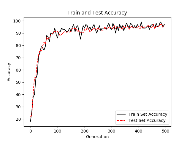
# 显示训练集和测试集上的准确率
plt.plot(eval_indices, train_acc, 'k-', label='Train Set Accuracy')
plt.plot(eval_indices, test_acc, 'r--', label='Test Set Accuracy')
plt.title('Train and Test Accuracy')
plt.xlabel('Generation')
plt.ylabel('Accuracy')
plt.legend(loc='lower right') # 显示标题出现的位置在图片右下角,否则不会显示标题
plt.show()
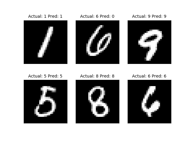
# 绘制样例图片
# 绘制最后一个batch中的6张图片
actuals = rand_y[0:6]
# print(actuals)[8 6 8 2 3 5]
predictions = np.argmax(temp_train_preds, axis=1)[0:6]
# 表示返回0~6个temp_train_preds中第一维数据中最大值所在位置
# print(predictions)[8 6 8 2 3 0]
images = np.squeeze(rand_x[0:6]) # 降维度,只保留有用的数据信息
Nrows = 2
Ncols = 3
fig = plt.figure() # 设置一个大的figure,向其中添加子图片
for i in range(6):
ax = fig.add_subplot(Nrows, Ncols, i + 1) # 设置当前图片所在位置
ax.imshow(np.reshape(images[i], [28, 28]), cmap='Greys_r') # 子块显示图片使用imshow语句
ax.set_title('Actual: ' + str(actuals[i]) + ' Pred: ' + str(predictions[i]), fontsize=10) # 设置子图标题
frame = plt.gca() # 去除图的边框
frame.axes.get_xaxis().set_visible(False) # 设置x坐标轴不可见
frame.axes.get_yaxis().set_visible(False) # 设置y坐标轴不可见
plt.show() # 显示figure
sess.close()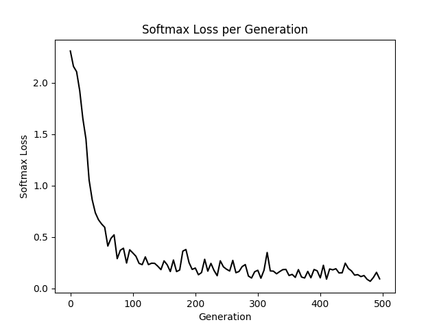

相关文章推荐
- Tensoflow+CNN实现简单的mnist手写数字识别
- Android+TensorFlow+CNN+MNIST 手写数字识别实现
- 卷积神经网络(CNN)的简单实现(MNIST)
- tensorflow mnist数据集 cnn demo
- Tensorflow CNN 的简单实现
- 卷积神经网络(CNN)的简单实现(MNIST)
- TensorFlow CNN 以库函数的方式实现MNIST手写识别
- TF:TF下CNN实现mnist数据集预测 96%采用placeholder用法+2层C及其max_pool法+隐藏层dropout法+输出层softmax法+目标函数cross_entropy法+A
- Android+TensorFlow+CNN+MNIST 手写数字识别实现
- TensorflowTutorial_一维数据构造简单CNN
- Android+TensorFlow+CNN+MNIST实现手写数字识别
- TensorflowTutorial_二维数据构造简单CNN
- tensorflow MNIST数据集上简单的MLP网络
- 卷积神经网络(CNN)的简单实现(MNIST)
- [转]卷积神经网络(CNN)的简单实现(MNIST)
- 卷积神经网络(CNN)的简单实现(MNIST)
- tensorflow 学习专栏(六):使用卷积神经网络(CNN)在mnist数据集上实现分类
- 【Tensorflow】用tersorflow内置函数做图片预处理
- TensorFlow在MNIST中的应用 识别手写数字(OpenCV+TensorFlow+CNN)
- 用tensorflow实现usps和mnist数据集的迁移学习