深度学习框架TensorFlow学习与应用（五）——TensorBoard结构与可视化

一、TensorBoard网络结构

先用pip3show tensorflow-tensorboard查看tensorboard是否已经安装

举例：

import tensorflow as tf
from tensorflow.examples.tutorials.mnist import input_data
#载入数据集
mnist=input_data.read_data_sets("D:\\MNIST_data",one_hot=True)
#每个批次的大小
batch_size=100
#计算一共有多少个批次
n_batch=int(mnist.train.num_examples/batch_size)

#命名空间
with tf.name_scope('input'):
#定义两个placeholder
x=tf.placeholder(tf.float32,[None,784],name='x-input')
y=tf.placeholder(tf.float32,[None,10],name='y-input')

with tf.name_scope('layer'):
#创建一个简单的神经网络
with tf.name_scope('wights'):
W=tf.Variable(tf.zeros([784,10]))
with tf.name_scope('biases'):
b=tf.Variable(tf.zeros([10]))
with tf.name_scope('xw_plus_b'):
wx_plus_b=tf.matmul(x,W)+b
with tf.name_scope('sofemax'):
prediction=tf.nn.softmax(tf.matmul(x,W)+b)

#二次代价函数
#loss=tf.reduce_mean(tf.square(y-prediction))
loss=tf.reduce_mean(tf.nn.softmax_cross_entropy_with_logits(labels=y,logits=prediction))
#使用梯度下降法
train_step=tf.train.GradientDescentOptimizer(0.2).minimize(loss)

#初始化变量
init=tf.global_variables_initializer()

#结果存放在一个布尔型列表中
correct_prediction=tf.equal(tf.argmax(y,1),tf.argmax(prediction,1))#比较两个参数大小，相同为true。argmax返回一维张量中最大的值所在的位置
#求准确率
accuracy=tf.reduce_mean(tf.cast(correct_prediction,tf.float32))#将布尔型转化为32位浮点型，再求一个平均值。true变为1.0，false变为0。

with tf.Session() as sess:
sess.run(init)
write=tf.summary.FileWriter('logs/',sess.graph)#在当前文件中写文件，存的就是图的结构
for epoch in range(1):
for batch in range(n_batch):
batch_xs,batch_ys=mnist.train.next_batch(batch_size)
sess.run(train_step,feed_dict={x:batch_xs,y:batch_ys})

acc=sess.run(accuracy,feed_dict={x:mnist.test.images,y:mnist.test.labels})
print("Iter "+str(epoch)+",Testing Accuracy "+str(acc))

1
2
3
4
5
6
7
8
9
10
11
12
13
14
15
16
17
18
19
20
21
22
23
24
25
26
27
28
29
30
31
32
33
34
35
36
37
38
39
40
41
42
43
44
45
46
47
48
49
50
运行后打开cmd（TensorFlow环境下）：

tensorboard --logdir=C:\Users\JLUTiger\logs #文件的路径

1
得到如下的信息：

TensorBoard 0.4.0rc2 at http://DESKTOP-UEGK0FV:6006 (Press CTRL+C to quit)

1
复制链接在浏览器中打开，便进入TensorBoard，如下所示：

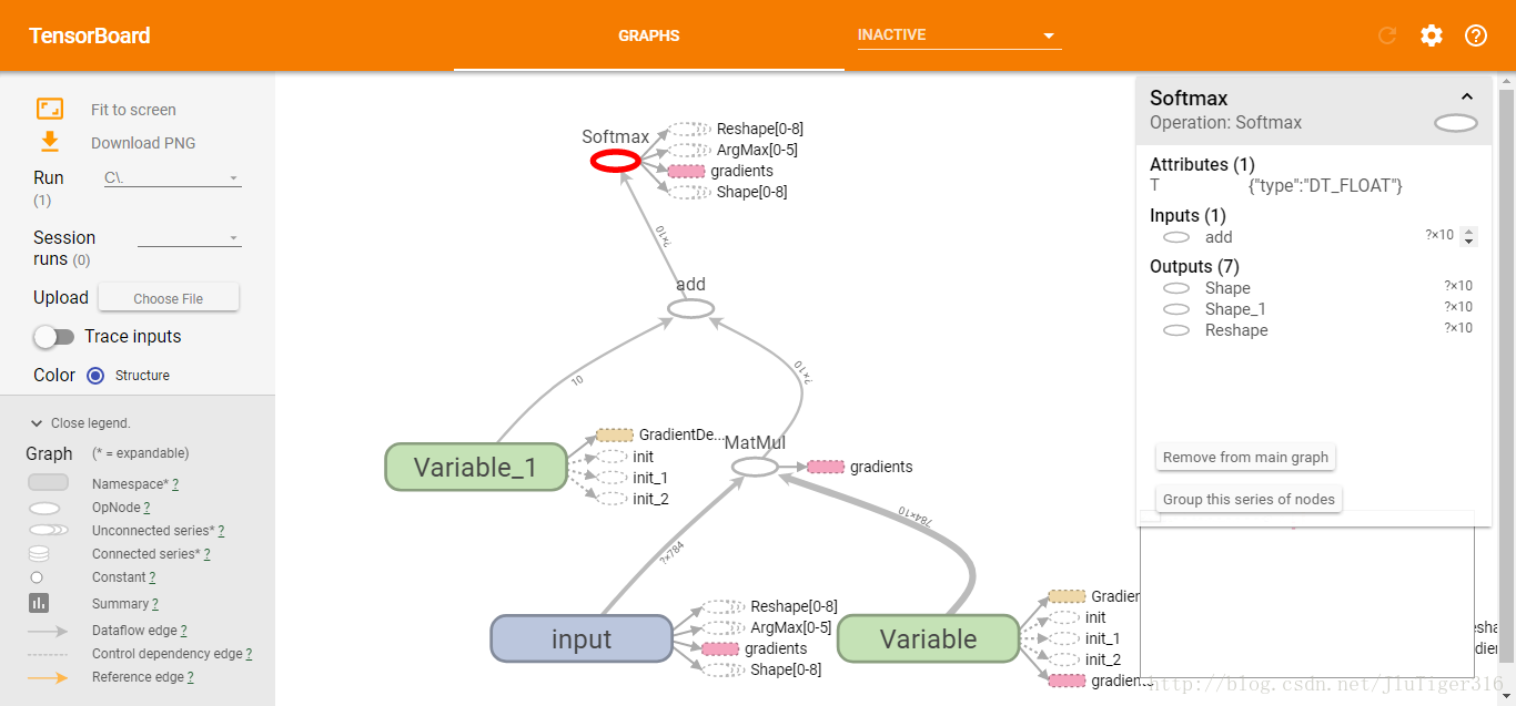
从TensorBoard中可以看出数据是怎么流动的等信息。

二、TensorBoard网络运行

将上面的代码改写为：

import tensorflow as tf
from tensorflow.examples.tutorials.mnist import input_data
#载入数据集
tf.reset_default_graph()
mnist=input_data.read_data_sets("D:\BaiDu\MNIST_data",one_hot=True)

#每个批次的大小
batch_size=100
#计算一共有多少个批次
n_batch=mnist.train.num_examples//batch_size

#参数概要
def variable_summaries(var):
with tf.name_scope('summaries'):
mean=tf.reduce_mean(var)
tf.summary.scalar('mean',mean)#平均值
with tf.name_scope('stddev'):
stddev=tf.sqrt(tf.reduce_mean(tf.square(var-mean)))
tf.summary.scalar('stddev',stddev)#标准差
tf.summary.scalar('max',tf.reduce_max(var))#最大值
tf.summary.scalar('min',tf.reduce_min(var))#最小值
tf.summary.histogram('histogram',var)#直方图

#命名空间
with tf.name_scope('input'):
#定义两个placeholder
x=tf.placeholder(tf.float32,[None,784],name='x-input')
y=tf.placeholder(tf.float32,[None,10],name='y-input')

with tf.name_scope('layer'):
#创建一个简单的神经网络
with tf.name_scope('wights'):
W=tf.Variable(tf.zeros([784,10]),name='W')
variable_summaries(W)
with tf.name_scope('biases'):
b=tf.Variable(tf.zeros([10]),name='b')
variable_summaries(b)
with tf.name_scope('xw_plus_b'):
wx_plus_b=tf.matmul(x,W)+b
with tf.name_scope('softmax'):
prediction=tf.nn.softmax(wx_plus_b)

#二次代价函数
#loss=tf.reduce_mean(tf.square(y-prediction))
with tf.name_scope('loss'):
loss=tf.reduce_mean(tf.nn.softmax_cross_entropy_with_logits(labels=y,logits=prediction))
tf.summary.scalar('loss',loss)
#使用梯度下降法
with tf.name_scope('train'):
train_step=tf.train.GradientDescentOptimizer(0.2).minimize(loss)

#初始化变量
init=tf.global_variables_initializer()
with tf.name_scope('accuracy'):
with tf.name_scope('correct_prediction'):
#结果存放在一个布尔型列表中
correct_prediction=tf.equal(tf.argmax(y,1),tf.argmax(prediction,1))#比较两个参数大小，相同为true。argmax返回一维张量中最大的值所在的位置
with tf.name_scope('accuracy'):
#求准确率
accuracy=tf.reduce_mean(tf.cast(correct_prediction,tf.float32))#将布尔型转化为32位浮点型，再求一个平均值。true变为1.0，false变为0。
tf.summary.scalar('accuracy',accuracy)

#合并所有的summary
merged=tf.summary.merge_all()

#以下的与结构没什么关系
with tf.Session() as sess:
sess.run(init)
writer=tf.summary.FileWriter('logs/',sess.graph)#在当前文件中写文件，存的就是图的结构
for epoch in range(51):
for batch in range(n_batch):
batch_xs,batch_ys=mnist.train.next_batch(batch_size)
summary,_=sess.run([merged,train_step],feed_dict={x:batch_xs,y:batch_ys})#每训练一次都统计一次

writer.add_summary(summary,epoch)

acc=sess.run(accuracy,feed_dict={x:mnist.test.images,y:mnist.test.labels})
print("Iter "+str(epoch)+",Testing Accuracy "+str(acc))

1
2
3
4
5
6
7
8
9
10
11
12
13
14
15
16
17
18
19
20
21
22
23
24
25
26
27
28
29
30
31
32
33
34
35
36
37
38
39
40
41
42
43
44
45
46
47
48
49
50
51
52
53
54
55
56
57
58
59
60
61
62
63
64
65
66
67
68
69
70
71
72
73
74
75
76
77
78
79
80
注意： 
起初运行时会报错：InvalidArgumentError: You must feed a value for placeholder tensor ‘inputs/x_input’ 。 
引用别人的方法： if you’re using IPython or Jupyter, it’ll cause that problem after running repeatedly.there are two main ways that you could fix that: 
A. 
tf.reset_default_graph() 
call firstly, before your tf operations code 
B. 
using 
with tf.Graph().as_default() as g: 
your tf operations code 
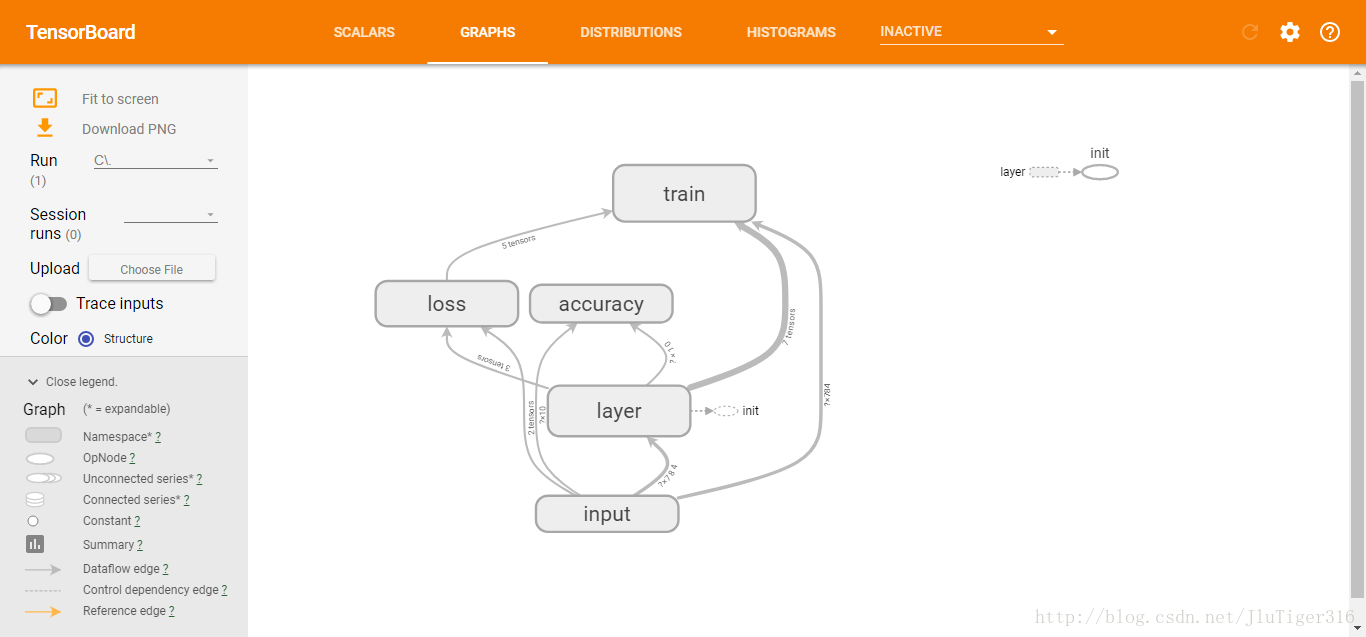
如果有别的错误也可以参考这篇博文：网络结构：

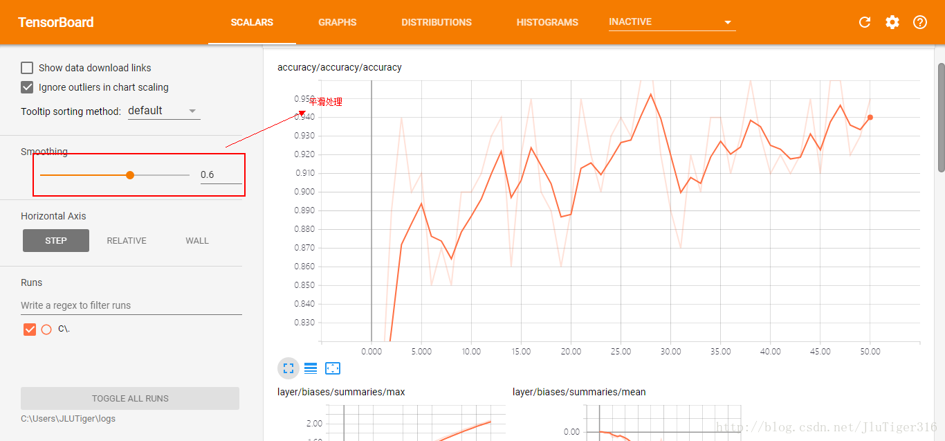
准确率：

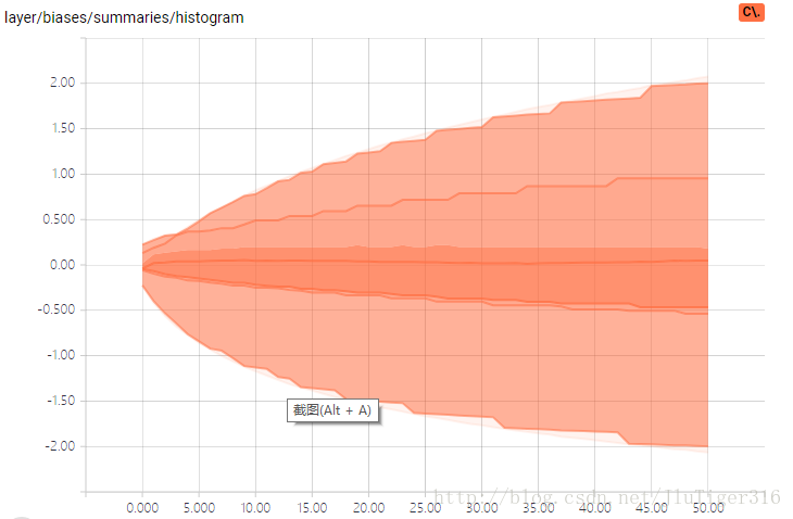
偏置值分布图：

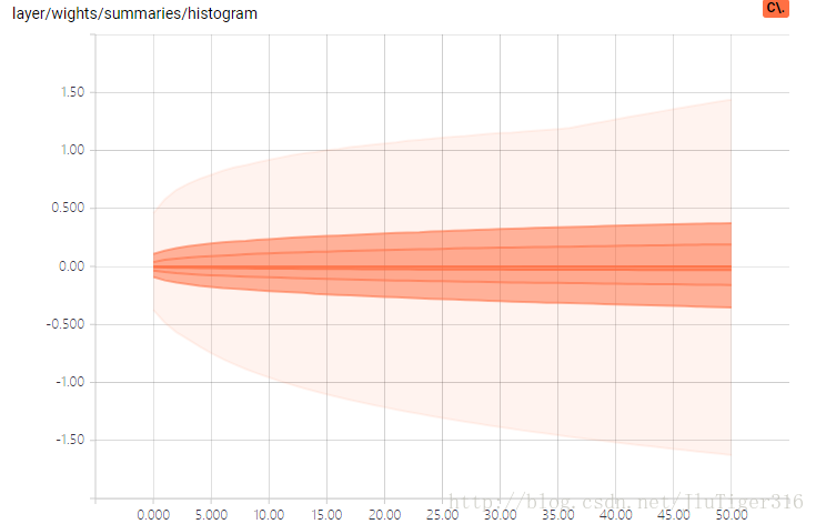
权值分布图：    颜色较深的地方表示分布比较集中


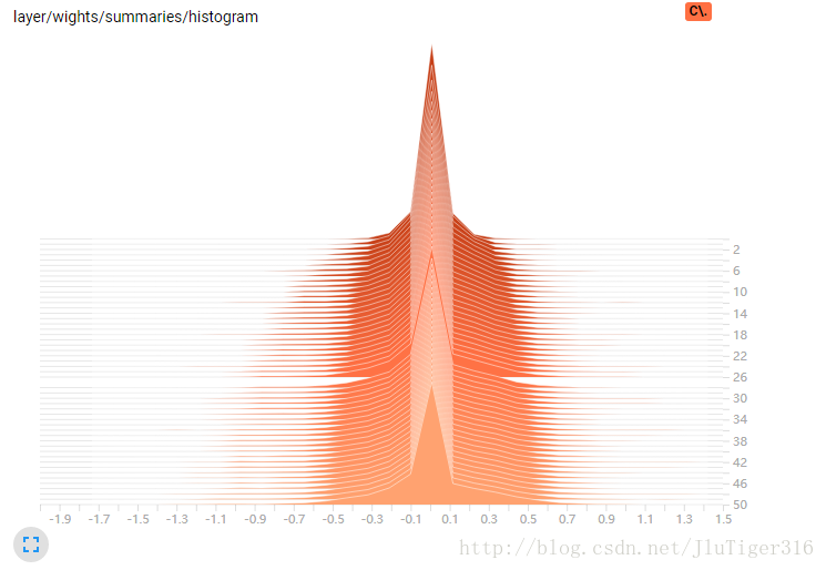
权值直方图：

如果感觉图中的点比较少，可以改用下列类似代码：

for i in range(2001):
#m每个批次100个样本
batch_xs,batch_xs=mnist.train.next_batch(100)
summary,_=sess.run([merged,train_step],feed_dict={x:batch_xs,y:batch_xs})
writer.add_summary(summary,i)
if i%500==0:
print(sess.run(accuracy,feed_dict={x:mnist.test.images,y:mnist.test.labels}))

1
2
3
4
5
6
7
通过查看TensorBoard中各个图像，可以分析出程序是否存在问题，从而便于进一步的优化改进。