CS231n课程作业(一) Two-layer Neural Network
2018-01-21 14:13
543 查看
神经网络的过程主要就是forward propagation和backward propagation。
forward propagation to evaluate score function & loss function, then back propagation 对每一层计算loss对W和b的梯度,利用梯度完成W和b的更新。
总体过程可以理解为:forward–>backward–>update–>forward–>backward–>update……
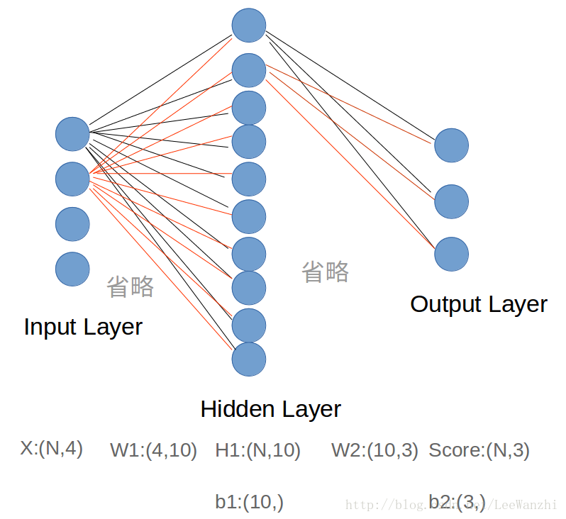
这是一个两层的full-connected神经网络,分别是输入层、隐藏层和输出层(输入层不算一层)。输入层4个节点表示样本是4维的,输出层3个节点表示有3类,输出的结果是每个类的score。
FC层(全连接层):每个神经元都连接上一层的所有神经元的layer。
在神经网络中,bigger = better,即网络模型越大越好。more neurons = more capacity,因为机器学习中经常出现模型表达能力不足的情况。
对于神经网络的更形象理解:
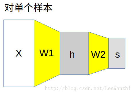
这里activation function采用的是ReLU函数。
Why we set activation function?
answer:如果不设置activation function,则每层的output都是input的线性函数,则无论隐藏层有多少层,都与没有隐藏层效果一样。因此,设置activation function,目的是为了对input进行非线性转化,然后output,使神经网络更有意义。
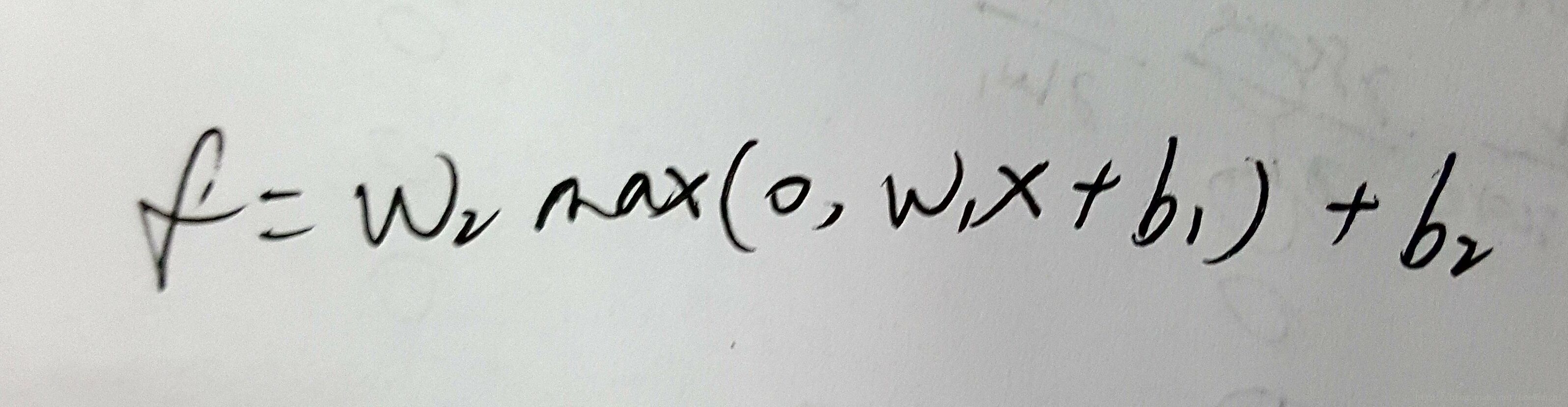
完成作业的关键仍是loss function对W求梯度。下面求gradient(注意:我在角标表示上有错误,但不影响理解和代码化):
这样,score、loss和gradient都表达出来了,2层神经网络也就可以完成了。
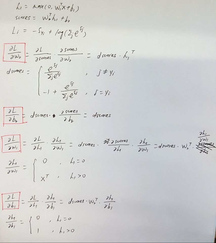
Backward:分别对W2、b2、W1、b1求梯度
然后check:
基本迭代过程是这样的:forward–>backward–>update–>forward–>backward–>update……
训练完模型,即可以对未知样本做出prediction。
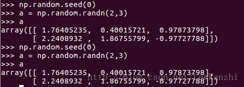
function: 选定固定的随机数,a为任意数字(如0)。即后面每次产生的随机数都固定。
2. np.nditer(array, flags=[‘multi_index’], op_flags=[‘readwrite’])
function: 构建一个迭代器。
参数1:数组; 参数2:多重索引; 参数3:可读写
本作业中,用于输出数组的index,从而进行数值梯度的计算。

forward propagation to evaluate score function & loss function, then back propagation 对每一层计算loss对W和b的梯度,利用梯度完成W和b的更新。
总体过程可以理解为:forward–>backward–>update–>forward–>backward–>update……
一、理论知识
1. 直观理解
这是一个两层的full-connected神经网络,分别是输入层、隐藏层和输出层(输入层不算一层)。输入层4个节点表示样本是4维的,输出层3个节点表示有3类,输出的结果是每个类的score。
FC层(全连接层):每个神经元都连接上一层的所有神经元的layer。
在神经网络中,bigger = better,即网络模型越大越好。more neurons = more capacity,因为机器学习中经常出现模型表达能力不足的情况。
对于神经网络的更形象理解:
2. score function
这里activation function采用的是ReLU函数。
Why we set activation function?
answer:如果不设置activation function,则每层的output都是input的线性函数,则无论隐藏层有多少层,都与没有隐藏层效果一样。因此,设置activation function,目的是为了对input进行非线性转化,然后output,使神经网络更有意义。
3. loss function及求梯度
本次作业中使用的是softmax loss function。可参考softmax classifier。完成作业的关键仍是loss function对W求梯度。下面求gradient(注意:我在角标表示上有错误,但不影响理解和代码化):
这样,score、loss和gradient都表达出来了,2层神经网络也就可以完成了。
二、Two-layer Neural Network
1. Forward Propagation & Backward Propagation
Forward: 计算score,再根据score计算lossBackward:分别对W2、b2、W1、b1求梯度
def loss(self, X, y=None, reg=0.0):
"""
Compute the loss and gradients for a two layer fully connected neural
network.

Inputs:
- X: Input data of shape (N, D). Each X[i] is a training sample.
- y: Vector of training labels. y[i] is the label for X[i], and each y[i] is
an integer in the range 0 <= y[i] < C. This parameter is optional; if it
is not passed then we only return scores, and if it is passed then we
instead return the loss and gradients.
- reg: Regularization strength.

Returns:
If y is None, return a matrix scores of shape (N, C) where scores[i, c] is
the score for class c on input X[i].

If y is not None, instead return a tuple of:
- loss: Loss (data loss and regularization loss) for this batch of training
samples.
- grads: Dictionary mapping parameter names to gradients of those parameters
with respect to the loss function; has the same keys as self.params.
"""
# Unpack variables from the params dictionary
W1, b1 = self.params['W1'], self.params['b1']
W2, b2 = self.params['W2'], self.params['b2']
N, D = X.shape

# Compute the forward pass
scores = None
#############################################################################
# TODO: Perform the forward pass, computing the class scores for the input. #
# Store the result in the scores variable, which should be an array of      #
# shape (N, C).                                                             #
#############################################################################
h1 = np.maximum(0, np.dot(X,W1) + b1) #(5,10)
#print (h1.shape)
scores = np.dot(h1,W2) + b2 # (5,3)
#print (scores.shape)
#############################################################################
#                              END OF YOUR CODE                             #
#############################################################################

# If the targets are not given then jump out, we're done
if y is None:
return scores

# Compute the loss
loss = None
#############################################################################
# TODO: Finish the forward pass, and compute the loss. This should include  #
# both the data loss and L2 regularization for W1 and W2. Store the result  #
# in the variable loss, which should be a scalar. Use the Softmax           #
# classifier loss.                                                          #
#############################################################################
exp_S = np.exp(scores) #(5,3)
sum_exp_S = np.sum(exp_S,axis = 1)
sum_exp_S = sum_exp_S.reshape(-1,1) #(5,1)
#print (sum_exp_S.shape)
loss = np.sum(-scores[range(N),list(y)]) + sum(np.log(sum_exp_S))
loss = loss / N + 0.5 * reg * np.sum(W1 * W1) +  0.5 * reg * np.sum(W2 * W2)
#print (loss)
#############################################################################
#                              END OF YOUR CODE                             #
#############################################################################

# Backward pass: compute gradients
grads = {}
#############################################################################
# TODO: Compute the backward pass, computing the derivatives of the weights #
# and biases. Store the results in the grads dictionary. For example,       #
# grads['W1'] should store the gradient on W1, and be a matrix of same size #
#############################################################################
'''
网络为4-10-3
对于第2层:input为h1(5,10)
W2:(10,3)
output为score:(5,3)
对于第1层:input为X(5,4)
W1(5,10)
output为h1(5,10)
'''
#---------------------------------#
dscores = np.zeros(scores.shape)
dscores[range(N),list(y)] = -1
dscores += (exp_S/sum_exp_S) #(5,3)
dscores /= N
grads['W2'] = np.dot(h1.T, dscores)
grads['W2'] += reg * W2
grads['b2'] = np.sum(dscores, axis = 0)
#---------------------------------#
dh1 = np.dot(dscores, W2.T)  #(5,10)
dh1_ReLU = (h1>0) * dh1
grads['W1'] = X.T.dot(dh1_ReLU) + reg * W1
grads['b1'] = np.sum(dh1_ReLU, axis = 0)
#---------------------------------#
'''
本人之前的写法:
缺点:无法很少的利用中间变量;
逻辑上可读性差
buf = np.zeros(scores.shape)
buf[range(N),list(y)] = -1
#print (buf+(exp_S/sum_exp_S))
grads['W2'] = np.dot(h1.T,(buf + (exp_S/sum_exp_S))) #(10,3)
grads['W2'] = grads['W2']/N + reg * W2
grads['b2'] = np.sum((exp_S/sum_exp_S)+buf, axis = 0) #(3,)

'''
#############################################################################
#                              END OF YOUR CODE                             #
#############################################################################

return loss, grads
2. Gradient Check
首先计算numeric gradient:def eval_numerical_gradient(f, x, verbose=True, h=0.00001): """ a naive implementation of numerical gradient of f at x - f should be a function that takes a single argument - x is the point (numpy array) to evaluate the gradient at """ fx = f(x) # evaluate function value at original point # x: 权重W1,W2,b2,b1 grad = np.zeros_like(x) # iterate over all indexes in x it = np.nditer(x, flags=['multi_index'], op_flags=['readwrite']) #构建一个迭代器 while not it.finished: # evaluate function at x+h ix = it.multi_index #输出结果为元素的索引 oldval = x[ix] #权重中的元素值 x[ix] = oldval + h # increment by h fxph = f(x) # evalute f(x + h) x[ix] = oldval - h fxmh = f(x) # evaluate f(x - h) x[ix] = oldval # restore # compute the partial derivative with centered formula grad[ix] = (fxph - fxmh) / (2 * h) # the slope if verbose: print(ix, grad[ix]) #输出数值梯度 it.iternext() # step to next dimension,如果不加这句话,则始终保持在(0,0) return grad #返回的是数值梯度
然后check:
from cs231n.gradient_check import eval_numerical_gradient

# Use numeric gradient checking to check your implementation of the backward pass.
# If your implementation is correct, the difference between the numeric and
# analytic gradients should be less than 1e-8 for each of W1, W2, b1, and b2.

loss, grads = net.loss(X, y, reg=0.1)
#print (loss)
#print (grads)
# these should all be less than 1e-8 or so
for param_name in grads:
f = lambda W: net.loss(X, y, reg=0.1)[0] #input:W; output:loss
param_grad_num = eval_numerical_gradient(f, net.params[param_name], verbose=False) #返回数值梯度
#print (np.abs(param_grad_num - grads[param_name]))
print('%s max relative error: %e' % (param_name, rel_error(param_grad_num, grads[param_name])))
3. Train a Network
既然forward和backward都已经完成了,且gradient检查通过,接下来就是训练出一个较好的模型。基本迭代过程是这样的:forward–>backward–>update–>forward–>backward–>update……
def train(self, X, y, X_val, y_val,
learning_rate=1e-3, learning_rate_decay=0.95,
reg=5e-6, num_iters=100,
batch_size=200, verbose=False):
"""
Train this neural network using stochastic gradient descent.

Inputs:
- X: A numpy array of shape (N, D) giving training data.
- y: A numpy array f shape (N,) giving training labels; y[i] = c means that
X[i] has label c, where 0 <= c < C.
- X_val: A numpy array of shape (N_val, D) giving validation data.
- y_val: A numpy array of shape (N_val,) giving validation labels.
- learning_rate: Scalar giving learning rate for optimization.
- learning_rate_decay: Scalar giving factor used to decay the learning rate
after each epoch.
- reg: Scalar giving regularization strength.
- num_iters: Number of steps to take when optimizing.
- batch_size: Number of training examples to use per step.
- verbose: boolean; if true print progress during optimization.
"""
num_train = X.shape[0]
iterations_per_epoch = max(num_train / batch_size, 1)

# Use SGD to optimize the parameters in self.model
loss_history = []
train_acc_history = []
val_acc_history = []

for it in xrange(num_iters):
X_batch = None
y_batch = None

#########################################################################
# TODO: Create a random minibatch of training data and labels, storing  #
# them in X_batch and y_batch respectively.                             #
#########################################################################
mask = np.random.choice(num_train,batch_size,replace = True)
X_batch = X[mask]
y_batch = y[mask]
#########################################################################
#                             END OF YOUR CODE                          #
#########################################################################

# Compute loss and gradients using the current minibatch
loss, grads = self.loss(X_batch, y=y_batch, reg=reg)
loss_history.append(loss)

#########################################################################
# TODO: Use the gradients in the grads dictionary to update the         #
# parameters of the network (stored in the dictionary self.params)      #
# using stochastic gradient descent. You'll need to use the gradients   #
# stored in the grads dictionary defined above.                         #
#########################################################################
self.params['W1'] += -learning_rate * grads['W1']
self.params['b1'] += -learning_rate * grads['b1']
self.params['W2'] += -learning_rate * grads['W2']
self.params['b2'] += -learning_rate * grads['b2']
#########################################################################
#                             END OF YOUR CODE                          #
#########################################################################

if verbose and it % 100 == 0:
print('iteration %d / %d: loss %f' % (it, num_iters, loss))

# Every epoch, check train and val accuracy and decay learning rate.
if it % iterations_per_epoch == 0:
# Check accuracy
#print ('第%d个epoch' %it)
train_acc = (self.predict(X_batch) == y_batch).mean()
val_acc = (self.predict(X_val) == y_val).mean()
train_acc_history.append(train_acc)
val_acc_history.append(val_acc)

# Decay learning rate
learning_rate *= learning_rate_decay #减小学习率

return {
'loss_history': loss_history,
'train_acc_history': train_acc_history,
'val_acc_history': val_acc_history,
}
训练完模型,即可以对未知样本做出prediction。
三、涉及到的numpy重要函数
1. np.random.seed(a)function: 选定固定的随机数,a为任意数字(如0)。即后面每次产生的随机数都固定。
2. np.nditer(array, flags=[‘multi_index’], op_flags=[‘readwrite’])
function: 构建一个迭代器。
参数1:数组; 参数2:多重索引; 参数3:可读写
本作业中,用于输出数组的index,从而进行数值梯度的计算。

相关文章推荐
- cs231n:assignment1——Q4: Two-Layer Neural Network
- CS231n课程作业(二) Multi-Layer Net、BN、Dropout、Optimization
- CS231n assignment1 -- Two-layer neural network
- Building+your+Deep+Neural+Network+-+Step+by+Step+v5 课程一第四周编程作业 1
- CS231N assignment1——Two-Layer Neural Network
- [CS231n@Stanford] Assignment1-Q4 (python) Two layer neural network实现
- ufldl学习笔记与编程作业:Multi-Layer Neural Network(多层神经网络+识别手写体编程)
- cs231n作业1--two_layer_net
- Andrew Ng 深度学习课程Deeplearning.ai 编程作业——deep Neural network for image classification(1-4.2)
- ufldl学习笔记与编程作业:Multi-Layer Neural Network(多层神经网络+识别手写体编程)
- DeepLearing学习笔记-Deep Neural Network在图像分类上的应用(第四周-作业2)
- 李飞飞CS231n课程-中文笔记(包括课后作业要求)翻译汇总
- sybase连接问题:ct_connect(): network packet layer: internal net library error: Net-Lib protocol driver call to connect two endpoints
- 【转】Principles of training multi-layer neural network using backpropagation
- CS231N-Lecture6 Training Neural Network part-2
- CS231n(2):课程作业# 1简介
- Hinton Neural Network课程笔记10a:融合模型Ensemble, Boosting, Bagging
- Multi-Layer Neural Network
- CS231n(3):课程作业# 2简介