进化策略
2018-01-14 19:31
113 查看
参考链接:
https://morvanzhou.github.io/tutorials/machine-learning/evolutionary-algorithm/3-01-evolution-strategy/
https://morvanzhou.github.io/tutorials/machine-learning/evolutionary-algorithm/3-00-evolution-strategy/
父代母代的 DNA 不用再是 01的这种形式, 用实数来代替,抛开了二进制的转换问题, 从而能解决实际生活中的很多由实数组成的真实问题. 比如我有一个关于 x 的公式, 而这个公式中其他参数, 我都能用 DNA 中的实数代替, 然后进化我的 DNA, 也就是优化这个公式. 这样用起来, 的确比遗传算法方便.
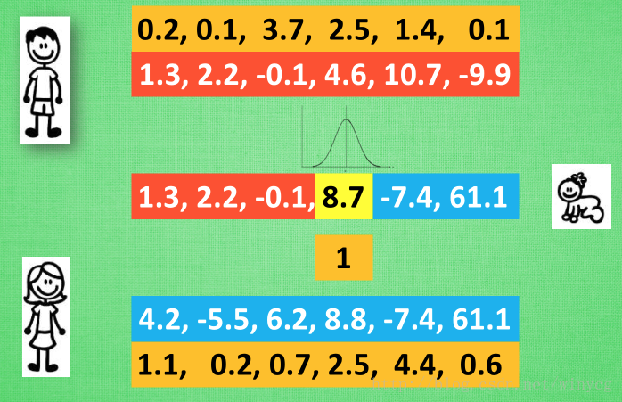
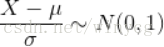
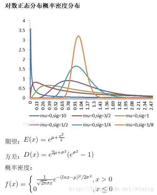
变异方法:遗传算法中简单的翻牌做法在这里行不通,于是引进变异强度的概念。 简单来说, 我们将父母代遗传下来的值看做是正态分布的平均值, 再在这个平均值上附加一个标准差, 我们就能用正态分布产生一个相近的数.
比如在这个8.8位置上的变异强度为1, 我们就按照1的标准差和8.8的均值产生一个离8.8的比较近的数, 比如8.7. 变异强度也可以被当成一组遗传信息从父母代的 DNA 中遗传下来,遗传给子代的变异强度基因也能变异.
总结:父母代有2种信息传递给后代:一种是记录所有位置的均值, 一种是记录这个均值的变异强度
与遗传算法的区别:
(1)选出优秀父母进行繁殖;先繁殖再选优秀的父母和子代
(2)用二进制编码DNA;DNA就是实数
(3)变异:通过0和1互相变化;通过正态分布变异
初始时,产生DNA值为[0,5]之间的数值,变异强度为[0,1]
产生子代:每次从种群中选择父代和母代进行交叉配对,产生1个子代个体,然后子代个体进行变异,包括变异强度的变异和DNA值得变异。
变异强度变异:变异强度在[-0.5,0.5]的范围内波动,且必须要大于0
DNA值变异:以原DNA值为均值,变异强度为标准差产生符合正态分布的随机数
淘汰个体保持种群个数:将产生的子代与父母代种群合并,并按个体的适应度进行排序,选出前population_size个个体作为进化后的一代
import numpy as np
import random
import matplotlib.pyplot as plt
population_size = 100
n_generations = 300
DNA_length = 1
x_bound = [0, 5]
n_children = 50
fig = plt.figure()
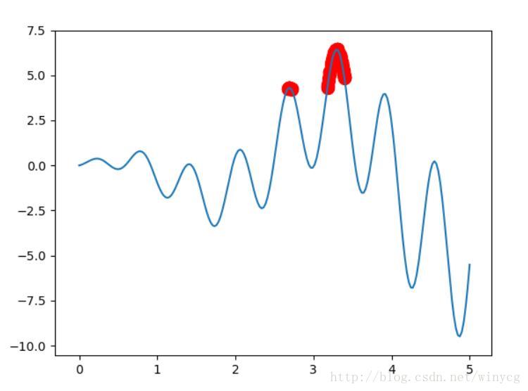
def F(x):
return np.sin(10*x)*x + np.cos(2*x)*x
class ES(object):
def __init__(self):
self.populations = {'DNA': 5 * np.random.rand(population_size, DNA_length),
'mutation': np.random.rand(population_size, DNA_length)}
def calculate_fitness(self):
return F(self.populations['DNA']).flatten()
def make_children(self):
children = {'DNA': np.empty((n_children, DNA_length)),
'mutation': np.empty((n_children, DNA_length))}
for i in range(n_children):
p1, p2 = np.random.choice(np.arange(population_size), (2,), replace=False)
crossover_points = np.random.randint(0, 1, (DNA_length,), dtype=np.bool)
children['DNA'][i][crossover_points] = self.populations['DNA'][p1][crossover_points]
children['DNA'][i][~crossover_points] = self.populations['DNA'][p2][~crossover_points]
children['mutation'][i][crossover_points] = self.populations['mutation'][p1][crossover_points]
children['mutation'][i][~crossover_points] = self.populations['mutation'][p2][~crossover_points]
# 使用正态分布变异
children['mutation'] = np.maximum(children['mutation']+random.random()-0.5, 0)
children['DNA'] = children['DNA']+np.random.randn(n_children, DNA_length)*children['mutation']
children['DNA'] = children['DNA'].clip(x_bound[0], x_bound[1])
return children
def eliminate_children(self, children):
self.populations['DNA'] = np.vstack((children['DNA'], self.populations['DNA']))
self.populations['mutation'] = np.vstack((children['mutation'], self.populations['mutation']))
fitness = self.calculate_fitness()
new_population_id = np.argsort(fitness)[-population_size:]
self.populations['DNA'] = self.populations['DNA'][new_population_id]
self.populations['mutation'] = self.populations['mutation'][new_population_id]
def evolve(self):
children = self.make_children()
self.eliminate_children(children)
population_value = np.linspace(x_bound[0], x_bound[1], 200)
plt.plot(population_value, F(population_value))
ga = ES()
for step in range(n_generations):
x = ga.populations['DNA'].flatten()
y = ga.calculate_fitness()
# 描点
# globals以字典类型返回当前位置的全部全局变量
if 'sca' in globals():
sca.remove()
sca = plt.scatter(x, y, s=100, c='red')
plt.pause(0.01)
ga.evolve()
plt.show()
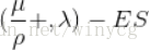
μ表示种群数量,ρ表示从种群中选取的用来繁殖子代的个体数量,λ表示生成子代的数量。如果是‘+’,表示将ρ和λ合起来进行适者生存,如果是‘,’,表示只对λ进行适者生存。以求上述的函数最大值为例。种群产生:种群中只有一个个体,有DNA值和变异强度两个参数产生子代:该个体通过正态分布变异产生一个个体,对应只有DNA值淘汰子代:比较父代和子代的fitness,保留大者,并根据公式改变变异强度
其中,σ是正态分布中的标准差,也就是变异强度
∂f
NES是一种使用适应度来诱导梯度下降的方法,具体过程如下:
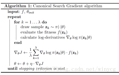
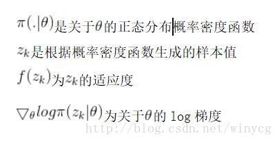
误差中加入了适应度f,使得适应度大的个体梯度下降的更多。也就是在一批数据中,如果适应度大的个体多,则这轮训练下降的梯度要多。
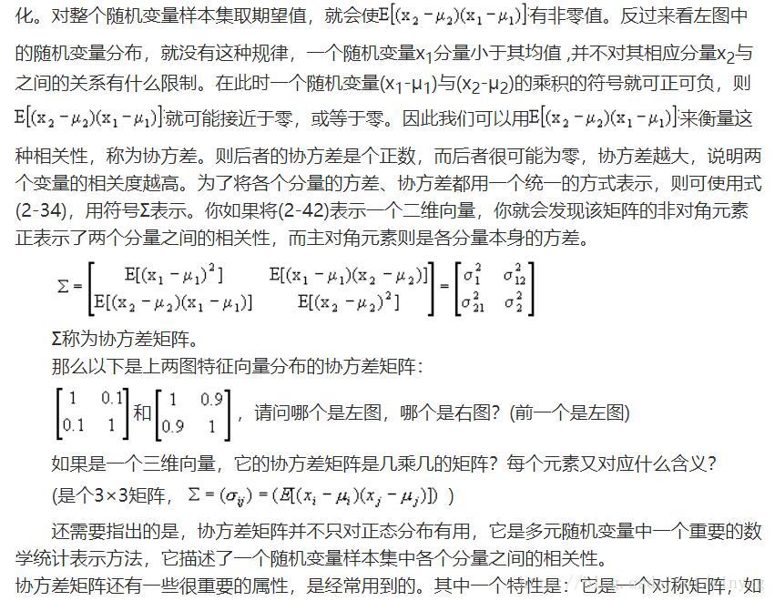
多元正态分布相关知识:http://www.360doc.com/content/11/0306/10/6165138_98561592.shtml
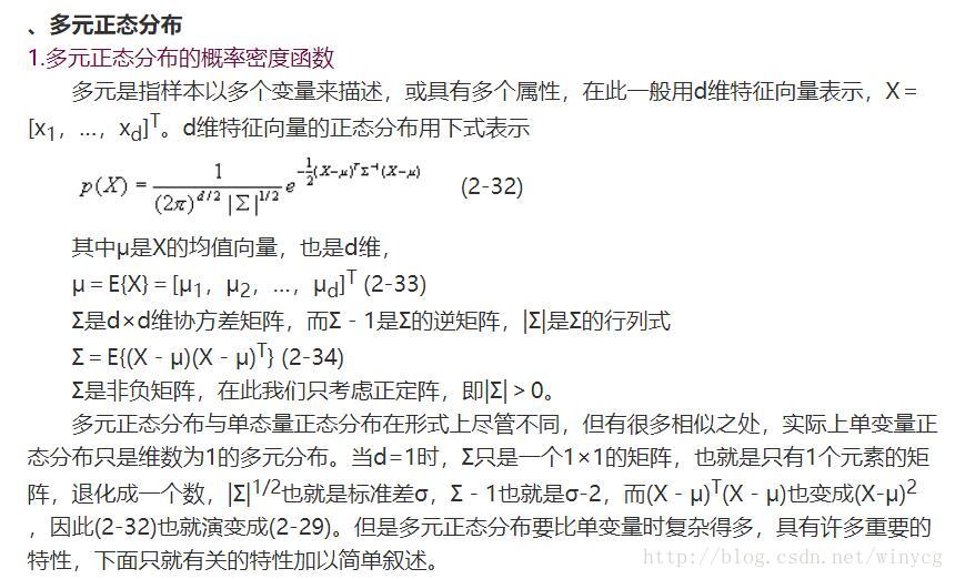
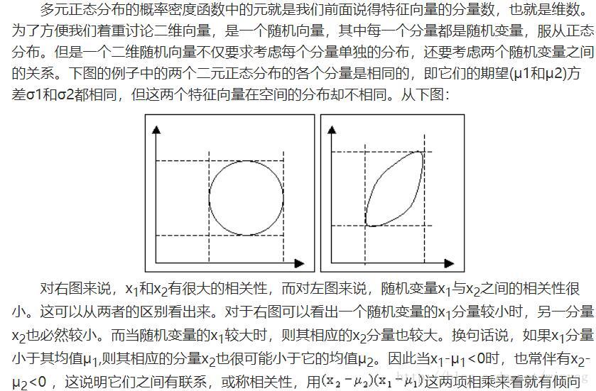

实例:使用二元正态分布使得x,y轴产生的点趋向于0
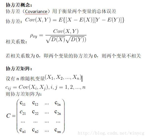
使用NES算法解决上述问题,需要优化两个正态分布的参数,分别为两个正态分布的均值mean和协方差矩阵cov。两个正态分布对应x轴和y轴产生数据。
该程序在迭代的过程中可能会报错,因为协方差矩阵在优化的过程中会变得不正定。
import numpy as np
import matplotlib.pyplot as plt
import tensorflow as tf
from tensorflow.contrib.distributions import MultivariateNormalFullCovariance
n_generations = 50
population_size = 20
DNA_length = 2
n_children = 1
lr = 0.1
fig = plt.figure()
# 初始生成13左右位置的点,离(0,0)较远,使得移动过程更明显
mean = tf.Variable(tf.random_normal([2, ], 13, 1), dtype=tf.float32)
# 协方差初始化需要测试,不同的值得效果差异较大
cov = tf.Variable(5 * tf.eye(DNA_length), dtype=tf.float32)
# 多元正态分布,传入初始化的均值和协方差
mvn = MultivariateNormalFullCovariance(loc=mean, covariance_matrix=cov)
# 用当前的多元正态分布生成训练数据
make_population = mvn.sample(population_size)
population = tf.placeholder(tf.float32, [population_size, DNA_length])
fitness = tf.placeholder(tf.float32, [population_size])
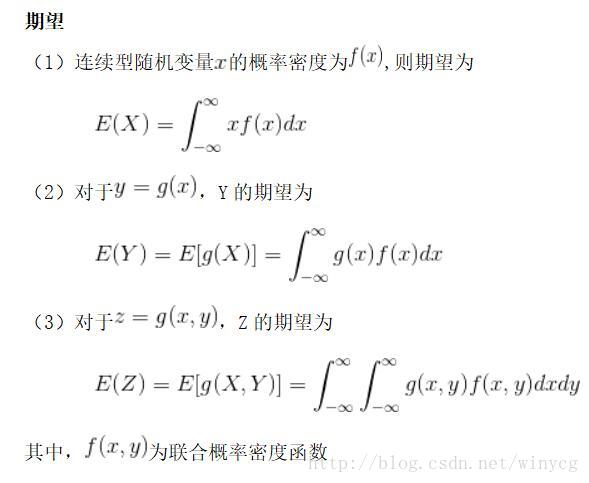
# 误差为该点的概率密度乘该点的适应度
loss = -tf.reduce_mean(mvn.log_prob(population) * fitness)
train_op = tf.train.GradientDescentOptimizer(lr).minimize(loss)
sess = tf.Session()
sess.run(tf.global_variables_initializer())
def show_contourf():
axis = np.linspace(-20, 20, 200)
X, Y = np.meshgrid(axis, axis)
Z = np.zeros_like(X)
for i in range(200):
for j in range(200):
Z[i][j] = -(X[i][j] ** 2 + Y[i][j] ** 2)
plt.contourf(X, Y, Z)
plt.xlim(-20, 20)
plt.ylim(-20, 20)
show_contourf()
for step in range(n_generations):
train_population = sess.run(make_population)
# 适应度为距离原点越近,适应度越大
train_fitness = -(train_population[:, 0] ** 2 + train_population[:, 1] ** 2)
sess.run(train_op, feed_dict={population: train_population,
fitness: train_fitness})
if 'sca' in globals():
sca.remove()
sca = plt.scatter(train_population[:, 0], train_population[:, 1], 30, 'k')
plt.pause(0.01)
print(sess.run([mean, cov]))
print('mean_fitness: %.3f' % (np.mean(train_fitness)),
'loss: %.3f' % (sess.run(loss, feed_dict={population: train_population,
fitness: train_fitness})))
plt.show()
https://morvanzhou.github.io/tutorials/machine-learning/evolutionary-algorithm/3-01-evolution-strategy/
https://morvanzhou.github.io/tutorials/machine-learning/evolutionary-algorithm/3-00-evolution-strategy/
进化策略(Evolution Strategy)
父代母代的 DNA 不用再是 01的这种形式, 用实数来代替,抛开了二进制的转换问题, 从而能解决实际生活中的很多由实数组成的真实问题. 比如我有一个关于 x 的公式, 而这个公式中其他参数, 我都能用 DNA 中的实数代替, 然后进化我的 DNA, 也就是优化这个公式. 这样用起来, 的确比遗传算法方便.
变异方法:遗传算法中简单的翻牌做法在这里行不通,于是引进变异强度的概念。 简单来说, 我们将父母代遗传下来的值看做是正态分布的平均值, 再在这个平均值上附加一个标准差, 我们就能用正态分布产生一个相近的数.
比如在这个8.8位置上的变异强度为1, 我们就按照1的标准差和8.8的均值产生一个离8.8的比较近的数, 比如8.7. 变异强度也可以被当成一组遗传信息从父母代的 DNA 中遗传下来,遗传给子代的变异强度基因也能变异.
总结:父母代有2种信息传递给后代:一种是记录所有位置的均值, 一种是记录这个均值的变异强度
与遗传算法的区别:
(1)选出优秀父母进行繁殖;先繁殖再选优秀的父母和子代
(2)用二进制编码DNA;DNA就是实数
(3)变异:通过0和1互相变化;通过正态分布变异
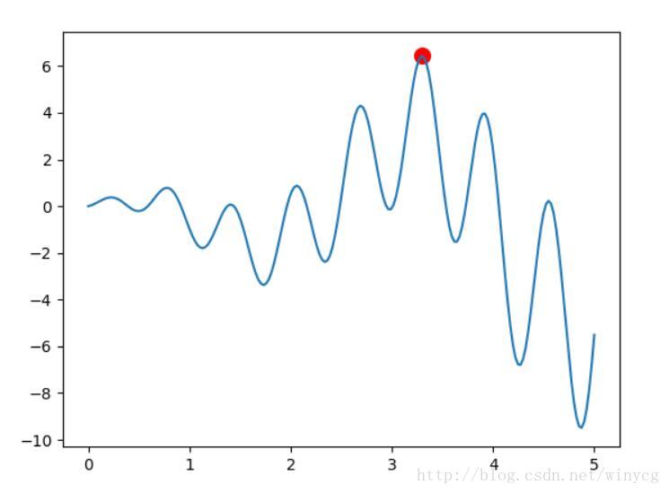
利用ES求解函数的最大值
种群产生:种群分为DNA值和变异强度两个属性值,DNA值表示函数的x值,变异强度为变异时的参数,产生后代的步骤细说。初始时,产生DNA值为[0,5]之间的数值,变异强度为[0,1]
产生子代:每次从种群中选择父代和母代进行交叉配对,产生1个子代个体,然后子代个体进行变异,包括变异强度的变异和DNA值得变异。
变异强度变异:变异强度在[-0.5,0.5]的范围内波动,且必须要大于0
DNA值变异:以原DNA值为均值,变异强度为标准差产生符合正态分布的随机数
淘汰个体保持种群个数:将产生的子代与父母代种群合并,并按个体的适应度进行排序,选出前population_size个个体作为进化后的一代
import numpy as np
import random
import matplotlib.pyplot as plt
population_size = 100
n_generations = 300
DNA_length = 1
x_bound = [0, 5]
n_children = 50
fig = plt.figure()
def F(x):
return np.sin(10*x)*x + np.cos(2*x)*x
class ES(object):
def __init__(self):
self.populations = {'DNA': 5 * np.random.rand(population_size, DNA_length),
'mutation': np.random.rand(population_size, DNA_length)}
def calculate_fitness(self):
return F(self.populations['DNA']).flatten()
def make_children(self):
children = {'DNA': np.empty((n_children, DNA_length)),
'mutation': np.empty((n_children, DNA_length))}
for i in range(n_children):
p1, p2 = np.random.choice(np.arange(population_size), (2,), replace=False)
crossover_points = np.random.randint(0, 1, (DNA_length,), dtype=np.bool)
children['DNA'][i][crossover_points] = self.populations['DNA'][p1][crossover_points]
children['DNA'][i][~crossover_points] = self.populations['DNA'][p2][~crossover_points]
children['mutation'][i][crossover_points] = self.populations['mutation'][p1][crossover_points]
children['mutation'][i][~crossover_points] = self.populations['mutation'][p2][~crossover_points]
# 使用正态分布变异
children['mutation'] = np.maximum(children['mutation']+random.random()-0.5, 0)
children['DNA'] = children['DNA']+np.random.randn(n_children, DNA_length)*children['mutation']
children['DNA'] = children['DNA'].clip(x_bound[0], x_bound[1])
return children
def eliminate_children(self, children):
self.populations['DNA'] = np.vstack((children['DNA'], self.populations['DNA']))
self.populations['mutation'] = np.vstack((children['mutation'], self.populations['mutation']))
fitness = self.calculate_fitness()
new_population_id = np.argsort(fitness)[-population_size:]
self.populations['DNA'] = self.populations['DNA'][new_population_id]
self.populations['mutation'] = self.populations['mutation'][new_population_id]
def evolve(self):
children = self.make_children()
self.eliminate_children(children)
population_value = np.linspace(x_bound[0], x_bound[1], 200)
plt.plot(population_value, F(population_value))
ga = ES()
for step in range(n_generations):
x = ga.populations['DNA'].flatten()
y = ga.calculate_fitness()
# 描点
# globals以字典类型返回当前位置的全部全局变量
if 'sca' in globals():
sca.remove()
sca = plt.scatter(x, y, s=100, c='red')
plt.pause(0.01)
ga.evolve()
plt.show()
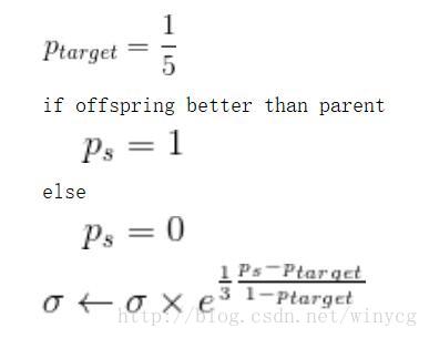
(1+1)-ES
首先解释一下这种形式的含义:通式:μ表示种群数量,ρ表示从种群中选取的用来繁殖子代的个体数量,λ表示生成子代的数量。如果是‘+’,表示将ρ和λ合起来进行适者生存,如果是‘,’,表示只对λ进行适者生存。以求上述的函数最大值为例。种群产生:种群中只有一个个体,有DNA值和变异强度两个参数产生子代:该个体通过正态分布变异产生一个个体,对应只有DNA值淘汰子代:比较父代和子代的fitness,保留大者,并根据公式改变变异强度
其中,σ是正态分布中的标准差,也就是变异强度
import numpy as np
import random
import matplotlib.pyplot as plt

n_generations = 300
DNA_length = 1
x_bound = [0, 5]
n_children = 1
fig = plt.figure()

def F(x):
return np.sin(10*x)*x + np.cos(2*x)*x

class ES(object):
def __init__(self):
# 初始化变异强度为2,因为初始离最优解可能较远
# 2是根据x的范围为[0,2]
self.populations = {'DNA': 5 * random.random(),
'mutation': 2}

def calculate_fitness(self, x):
return F(x)

def make_child(self):
child = {}
child['DNA'] = self.populations['DNA'] + \
self.populations['mutation'] * random.normalvariate(0, 1)
# np.clip()也可以对整数进行限定范围
child['DNA'] = np.clip(child['DNA'], x_bound[0], x_bound[1])
return child

def eliminate_child(self, child):
parent_fitness = self.calculate_fitness(self.populations['DNA'])
child_fitness = self.calculate_fitness(child['DNA'])
p_target = 1/5
if child_fitness > parent_fitness:
ps = 1
self.populations['DNA'] = child['DNA']
else:
ps = 0
self.populations['mutation'] = np.exp(1/3 * (ps - p_target)/(1 - p_target))

def evolve(self):
child = self.make_child()
self.eliminate_child(child)
# 返回生成的child用于画图
return child

population_value = np.linspace(x_bound[0], x_bound[1], 200)
plt.plot(population_value, F(population_value))

ga = ES()
for step in range(n_generations):
ga.evolve()
parent_x = ga.populations['DNA']
parent_y = ga.calculate_fitness(parent_x)
sca_parent = plt.scatter(parent_x, parent_y, s=100, c='red')
plt.pause(0.01)
if step != n_generations-1:
sca_parent.remove()
plt.show()
NES(Natural evolution strategies)
知识回顾:∂f
NES是一种使用适应度来诱导梯度下降的方法,具体过程如下:
误差中加入了适应度f,使得适应度大的个体梯度下降的更多。也就是在一批数据中,如果适应度大的个体多,则这轮训练下降的梯度要多。
多元正态分布相关知识:http://www.360doc.com/content/11/0306/10/6165138_98561592.shtml
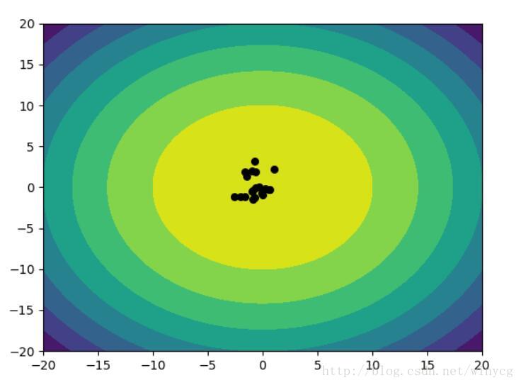
实例:使用二元正态分布使得x,y轴产生的点趋向于0
使用NES算法解决上述问题,需要优化两个正态分布的参数,分别为两个正态分布的均值mean和协方差矩阵cov。两个正态分布对应x轴和y轴产生数据。
该程序在迭代的过程中可能会报错,因为协方差矩阵在优化的过程中会变得不正定。
import numpy as np
import matplotlib.pyplot as plt
import tensorflow as tf
from tensorflow.contrib.distributions import MultivariateNormalFullCovariance
n_generations = 50
population_size = 20
DNA_length = 2
n_children = 1
lr = 0.1
fig = plt.figure()
# 初始生成13左右位置的点,离(0,0)较远,使得移动过程更明显
mean = tf.Variable(tf.random_normal([2, ], 13, 1), dtype=tf.float32)
# 协方差初始化需要测试,不同的值得效果差异较大
cov = tf.Variable(5 * tf.eye(DNA_length), dtype=tf.float32)
# 多元正态分布,传入初始化的均值和协方差
mvn = MultivariateNormalFullCovariance(loc=mean, covariance_matrix=cov)
# 用当前的多元正态分布生成训练数据
make_population = mvn.sample(population_size)
population = tf.placeholder(tf.float32, [population_size, DNA_length])
fitness = tf.placeholder(tf.float32, [population_size])
# 误差为该点的概率密度乘该点的适应度
loss = -tf.reduce_mean(mvn.log_prob(population) * fitness)
train_op = tf.train.GradientDescentOptimizer(lr).minimize(loss)
sess = tf.Session()
sess.run(tf.global_variables_initializer())
def show_contourf():
axis = np.linspace(-20, 20, 200)
X, Y = np.meshgrid(axis, axis)
Z = np.zeros_like(X)
for i in range(200):
for j in range(200):
Z[i][j] = -(X[i][j] ** 2 + Y[i][j] ** 2)
plt.contourf(X, Y, Z)
plt.xlim(-20, 20)
plt.ylim(-20, 20)
show_contourf()
for step in range(n_generations):
train_population = sess.run(make_population)
# 适应度为距离原点越近,适应度越大
train_fitness = -(train_population[:, 0] ** 2 + train_population[:, 1] ** 2)
sess.run(train_op, feed_dict={population: train_population,
fitness: train_fitness})
if 'sca' in globals():
sca.remove()
sca = plt.scatter(train_population[:, 0], train_population[:, 1], 30, 'k')
plt.pause(0.01)
print(sess.run([mean, cov]))
print('mean_fitness: %.3f' % (np.mean(train_fitness)),
'loss: %.3f' % (sess.run(loss, feed_dict={population: train_population,
fitness: train_fitness})))
plt.show()

相关文章推荐
- switch代码的进化 重构,至策略模式 工厂模式 插件模式 表驱动
- 基于L-System、遗传算法、人工生命进化模型的人工生命的计算机动画策略
- OpenAI详解进化策略方法:可替代强化学习
- 如何一文读懂「进化策略」?这里有几组动图!
- 从变分边界到进化策略,一文汇总机器学习变换技巧
- 《非零和时代》:人类历史发展与生物进化背后的基本的规律:环境恶劣,非零和的策略更容易生存 五星推荐
- 进化策略
- 进化策略
- 进化策略-python实现
- 特性开关之策略模式
- 设计模式原来如此-策略模式(Strategy Pattern)
- 关于阵列卡的配置参数Cache Policy(缓存策略)
- 内核文件加载执行控制方案实现(win7, win8 64位)--windows内核安全策略的演变
- Kafka源码深度解析-系列1 -消息队列的策略与语义
- Oracle数据库的安全策略
- 大OA平台策略修正OA技术缺陷
- 浅谈自己知道的首屏加载时间的优化策略
- 设计模式之五(策略模式)
- 雷观(二十):个人竞争策略,战国策与个人略