python 机器学习中模型评估和调参
2017-12-22 11:48
423 查看
在做数据处理时,需要用到不同的手法,如特征标准化,主成分分析,等等会重复用到某些参数,sklearn中提供了管道,可以一次性的解决该问题
先展示先通常的做法
先对数据标准化,然后做主成分分析降维,最后做回归预测
现在使用管道
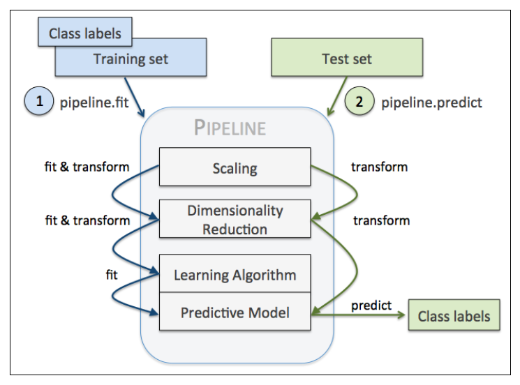
Pipeline对象接收元组构成的列表作为输入,每个元组第一个值作为变量名,元组第二个元素是sklearn中的transformer或Estimator。
管道中间每一步由sklearn中的transformer构成,最后一步是一个Estimator。我们的例子中,管道包含两个中间步骤,一个StandardScaler和一个PCA,这俩都是transformer,逻辑斯蒂回归分类器是Estimator。
当管道pipe_lr执行fit方法时,首先StandardScaler执行fit和transform方法,然后将转换后的数据输入给PCA,PCA同样执行fit和transform方法,最后将数据输入给LogisticRegression,训练一个LR模型。
对于管道来说,中间有多少个transformer都可以。工作方式如下
使用管道减少了很多代码量
现在回归模型的评估和调参
训练机器学习模型的关键一步是要评估模型的泛化能力。如果我们训练好模型后,还是用训练集取评估模型的性能,这显然是不符合逻辑的。一个模型如果性能不好,要么是因为模型过于复杂导致过拟合(高方差),要么是模型过于简单导致导致欠拟合(高偏差)。可是用什么方法评价模型的性能呢?这就是这一节要解决的问题,你会学习到两种交叉验证计数,holdout交叉验证和k折交叉验证, 来评估模型的泛化能力
一、holdout交叉验证(评估模型性能)
holdout方法很简单就是将数据集分为训练集和测试集,前者用于训练,后者用于评估
如果在模型选择的过程中,我们始终用测试集来评价模型性能,这实际上也将测试集变相地转为了训练集,这时候选择的最优模型很可能是过拟合的。
更好的holdout方法是将原始训练集分为三部分:训练集、验证集和测试集。训练机用于训练不同的模型,验证集用于模型选择。而测试集由于在训练模型和模型选择这两步都没有用到,对于模型来说是未知数据,因此可以用于评估模型的泛化能力。下图展示了holdout方法的步骤:
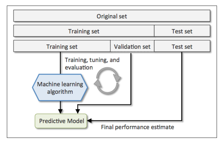
缺点:它对数据分割的方式很敏感,如果原始数据集分割不当,这包括训练集、验证集和测试集的样本数比例,以及分割后数据的分布情况是否和原始数据集分布情况相同等等。所以,不同的分割方式可能得到不同的最优模型参数
二、K折交叉验证(评估模型性能)
k折交叉验证的过程,第一步我们使用不重复抽样将原始数据随机分为k份,第二步 k-1份数据用于模型训练,剩下那一份数据用于测试模型。然后重复第二步k次,我们就得到了k个模型和他的评估结果(译者注:为了减小由于数据分割引入的误差,通常k折交叉验证要随机使用不同的划分方法重复p次,常见的有10次10折交叉验证)
然后我们计算k折交叉验证结果的平均值作为参数/模型的性能评估。使用k折交叉验证来寻找最优参数要比holdout方法更稳定。一旦我们找到最优参数,要使用这组参数在原始数据集上训练模型作为最终的模型。
k折交叉验证使用不重复采样,优点是每个样本只会在训练集或测试中出现一次,这样得到的模型评估结果有更低的方法。
下图演示了10折交叉验证:
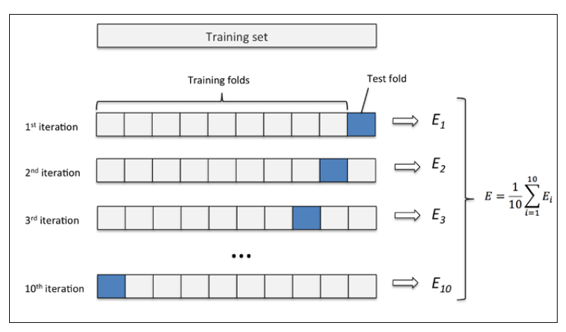
10次10折交叉验证我的理解是将按十种划分方法,每次将数据随机分成k分,k-1份训练,k份测试。获取十个模型和评估结果,然后取10次的平均值作为性能评估
更简单的方法
cv即k
三、学习曲线(调试算法)
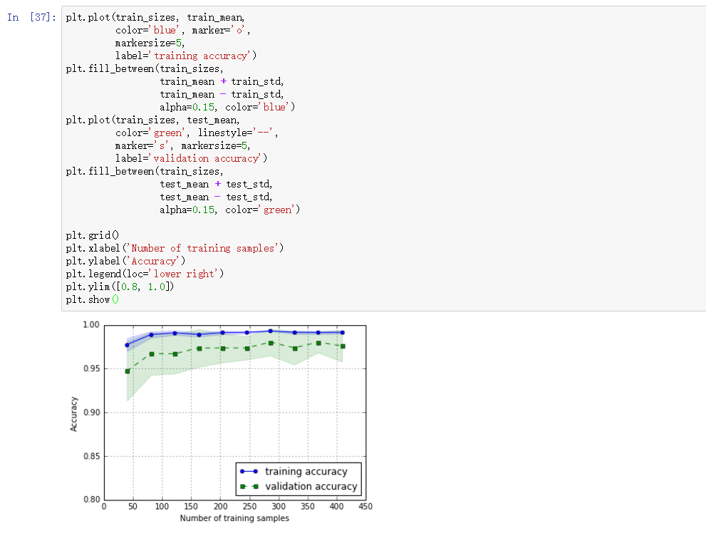
learning_curve中的train_sizes参数控制产生学习曲线的训练样本的绝对/相对数量,此处,我们设置的train_sizes=np.linspace(0.1, 1.0, 10),将训练集大小划分为10个相等的区间。learning_curve默认使用分层k折交叉验证计算交叉验证的准确率,我们通过cv设置k。
上图中可以看到,模型在测试集表现很好,不过训练集和测试集的准确率还是有一段小间隔,可能是模型有点过拟合
四、验证曲线解决过拟合和欠拟合(调试算法)
验证曲线和学习曲线很相近,不同的是这里画出的是不同参数下模型的准确率而不是不同训练集大小下的准确率
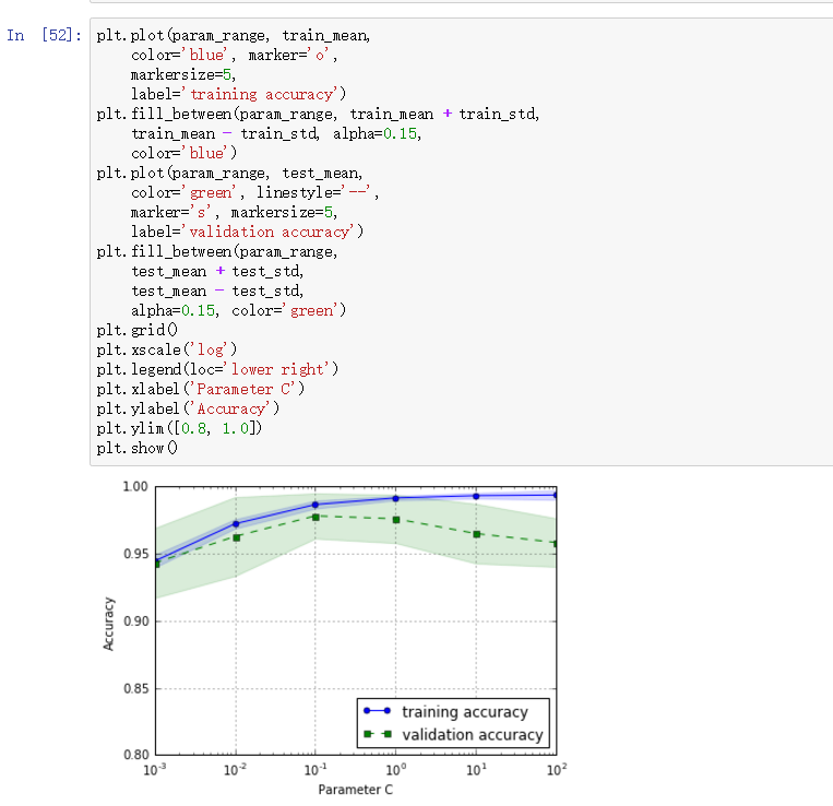
我们得到了参数C的验证曲线。
和learning_curve方法很像,validation_curve方法使用采样k折交叉验证来评估模型的性能。在validation_curve内部,我们设定了用来评估的参数,这里是C,也就是LR的正则系数的倒数。
观察上图,最好的C值是0.1。
总之,我们可以使用学习曲线判断算法是否拟合程度(欠拟合或者过拟合),然后使用验证曲线评估参数获取最好的参数
机器学习算法中有两类参数:从训练集中学习到的参数,比如逻辑斯蒂回归中的权重参数,另一类是模型的超参数,也就是需要人工设定的参数,比如正则项系数或者决策树的深度。
权重参数可以通过验证曲线来获取最好的参数,而超参数则可以使用网格搜索调参
五、网格搜索调参(调试算法)
网格搜索其实就是暴力搜索,事先为每个参数设定一组值,然后穷举各种参数组合,找到最好的那组
GridSearchCV中param_grid参数是字典构成的列表。对于线性SVM,我们只评估参数C;对于RBF核SVM,我们评估C和gamma。
最后, 我们通过best_parmas_得到最优参数组合。
sklearn人性化的一点是,我们可以直接利用最优参数建模(best_estimator_)
网格搜索虽然不错,但是穷举过于耗时,sklearn中还实现了随机搜索,使用 RandomizedSearchCV类,随机采样出不同的参数组合
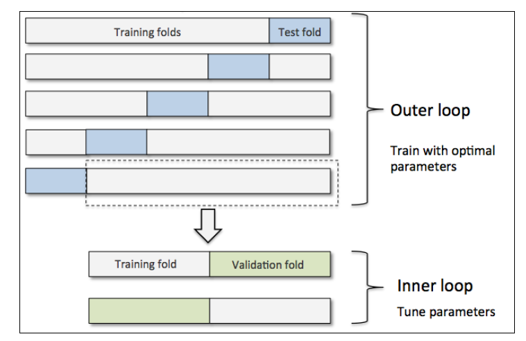
六、嵌套交叉验证(选择算法)
结合k折交叉验证和网格搜索是调参的好手段。可是如果我们想从茫茫算法中选择最合适的算法,用什么方法呢?这就是下面要介绍的嵌套交叉验证
嵌套交叉验证外层有一个k折交叉验证将数据分为训练集和测试集。还有一个内部交叉验证用于选择模型算法。下图演示了一个5折外层交叉沿则和2折内部交叉验证组成的嵌套交叉验证,也被称为5*2交叉验证
sklearn中如下使用嵌套交叉验证
svc的精确度
决策树分类器精确度
比较下两者的精确度,即可知道那种算法更加合适
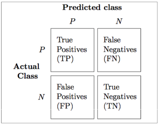
七、混淆矩阵(性能评价指标)
除了准确率,还有不少评价指标,如查准率,查全率,F1值等
混淆矩阵(confusion matrix), 能够展示学习算法表现的矩阵。混淆矩阵是一个平方矩阵,其中记录了一个分类器的TP(true positive)、TN(true negative)、FP(false positive)和FN(false negative):
python实现混淆矩阵
其实就是一个2*2的矩阵
TP实际为真,判断成功(判断为真)的个数
FN实际为真,判断错误(判断为假)
FP实际为假,判断错误(判断为真)
TN实际为假,判断成功(判断为假)
摘自https://www.gitbook.com/book/ljalphabeta/python-
先展示先通常的做法
import pandas as pd
from sklearn.preprocessing import StandardScaler
from sklearn.decomposition import PCA
from sklearn.linear_model import LogisticRegression

df = pd.read_csv('wdbc.csv')
X = df.iloc[:, 2:].values
y = df.iloc[:, 1].values
# 标准化
sc = StandardScaler()
X_train_std = sc.fit_transform(X_train)
X_test_std = sc.transform(X_test)
# 主成分分析PCA
pca = PCA(n_components=2)
X_train_pca = pca.fit_transform(X_train_std)
X_test_pca = pca.transform(X_test_std)
# 逻辑斯蒂回归预测
lr = LogisticRegression(random_state=1)
lr.fit(X_train_pca, y_train)
y_pred = lr.predict(X_test_pca)
先对数据标准化,然后做主成分分析降维,最后做回归预测
现在使用管道
from sklearn.pipeline import Pipeline

pipe_lr = Pipeline([('sc', StandardScaler()), ('pca', PCA(n_components=2)), ('lr', LogisticRegression(random_state=1))])
pipe_lr.fit(X_train, y_train)
pipe_lr.score(X_test, y_test)
Pipeline对象接收元组构成的列表作为输入,每个元组第一个值作为变量名,元组第二个元素是sklearn中的transformer或Estimator。
管道中间每一步由sklearn中的transformer构成,最后一步是一个Estimator。我们的例子中,管道包含两个中间步骤,一个StandardScaler和一个PCA,这俩都是transformer,逻辑斯蒂回归分类器是Estimator。
当管道pipe_lr执行fit方法时,首先StandardScaler执行fit和transform方法,然后将转换后的数据输入给PCA,PCA同样执行fit和transform方法,最后将数据输入给LogisticRegression,训练一个LR模型。
对于管道来说,中间有多少个transformer都可以。工作方式如下
使用管道减少了很多代码量
现在回归模型的评估和调参
训练机器学习模型的关键一步是要评估模型的泛化能力。如果我们训练好模型后,还是用训练集取评估模型的性能,这显然是不符合逻辑的。一个模型如果性能不好,要么是因为模型过于复杂导致过拟合(高方差),要么是模型过于简单导致导致欠拟合(高偏差)。可是用什么方法评价模型的性能呢?这就是这一节要解决的问题,你会学习到两种交叉验证计数,holdout交叉验证和k折交叉验证, 来评估模型的泛化能力
一、holdout交叉验证(评估模型性能)
holdout方法很简单就是将数据集分为训练集和测试集,前者用于训练,后者用于评估
如果在模型选择的过程中,我们始终用测试集来评价模型性能,这实际上也将测试集变相地转为了训练集,这时候选择的最优模型很可能是过拟合的。
更好的holdout方法是将原始训练集分为三部分:训练集、验证集和测试集。训练机用于训练不同的模型,验证集用于模型选择。而测试集由于在训练模型和模型选择这两步都没有用到,对于模型来说是未知数据,因此可以用于评估模型的泛化能力。下图展示了holdout方法的步骤:
缺点:它对数据分割的方式很敏感,如果原始数据集分割不当,这包括训练集、验证集和测试集的样本数比例,以及分割后数据的分布情况是否和原始数据集分布情况相同等等。所以,不同的分割方式可能得到不同的最优模型参数
二、K折交叉验证(评估模型性能)
k折交叉验证的过程,第一步我们使用不重复抽样将原始数据随机分为k份,第二步 k-1份数据用于模型训练,剩下那一份数据用于测试模型。然后重复第二步k次,我们就得到了k个模型和他的评估结果(译者注:为了减小由于数据分割引入的误差,通常k折交叉验证要随机使用不同的划分方法重复p次,常见的有10次10折交叉验证)
然后我们计算k折交叉验证结果的平均值作为参数/模型的性能评估。使用k折交叉验证来寻找最优参数要比holdout方法更稳定。一旦我们找到最优参数,要使用这组参数在原始数据集上训练模型作为最终的模型。
k折交叉验证使用不重复采样,优点是每个样本只会在训练集或测试中出现一次,这样得到的模型评估结果有更低的方法。
下图演示了10折交叉验证:
10次10折交叉验证我的理解是将按十种划分方法,每次将数据随机分成k分,k-1份训练,k份测试。获取十个模型和评估结果,然后取10次的平均值作为性能评估
from sklearn.model_selection import StratifiedKFold

pipe_lr = Pipeline([('sc', StandardScaler()), ('pca', PCA(n_components=2)), ('lr', LogisticRegression(random_state=1))])
pipe_lr.fit(X_train, y_train)
kfold = StratifiedKFold(y=y_train, n_folds=10, random_state=1)
scores= []
for k, (train, test) in enumerate(kfold):
pipe_lr.fit(X_train[train], y_train[train])
score = pipe_lr.score(X_train[test], y_train[test])
scores.append(scores)
print('Fold: %s, Class dist.: %s, Acc: %.3f' %(k+1, np.bincount(y_train[train]), score))print('CV accuracy: %.3f +/- %.3f' %(np.mean(scores), np.std(scores)))
更简单的方法
from sklearn.model_selection import StratifiedKFold

pipe_lr = Pipeline([('sc', StandardScaler()), ('pca', PCA(n_components=2)), ('lr', LogisticRegression(random_state=1))])
pipe_lr.fit(X_train, y_train)
scores = cross_val_score(estimator=pipe_lr, X=X_train, y=y_train, cv=10, n_jobs=1)
print('CV accuracy scores: %s' %scores)
print('CV accuracy: %.3f +/- %.3f' %(np.mean(scores), np.std(scores)))
cv即k
三、学习曲线(调试算法)
from sklearn.model_selection import learning_curve

pipe_lr = Pipeline([('scl', StandardScaler()), ('clf', LogisticRegression(penalty='l2', random_state=0))])
train_sizes, train_scores, test_scores = learning_curve(estimator=pipe_lr, X=X_train, y=y_train, train_sizes=np.linspace(0.1, 1.0, 10), cv=10, n_jobs=1)
train_mean = np.mean(train_scores, axis=1)
train_std = np.std(train_scores, axis=1)
test_mean = np.mean(test_scores, axis=1)
test_std = np.std(test_scores, axis=1)
plt.plot(train_sizes, train_mean, color='blue', marker='0', markersize=5, label='training accuracy')
plt.fill_between(train_sizes, train_mean + train_std, train_mean - train_std, alpha=0.15, color='blue')
plt.plot(train_sizes, test_mean, color='green', linestyle='--', marker='s', markersize=5, label='validation accuracy')
plt.fill_between(train_sizes, test_mean + test_std, test_mean - test_std, alpha=0.15, color='green')
plt.grid()
plt.xlabel('Number of training samples')
plt.ylabel('Accuracy')
plt.legend(loc='lower right')
plt.ylim([0.8, 1.0])
plt.show()
learning_curve中的train_sizes参数控制产生学习曲线的训练样本的绝对/相对数量,此处,我们设置的train_sizes=np.linspace(0.1, 1.0, 10),将训练集大小划分为10个相等的区间。learning_curve默认使用分层k折交叉验证计算交叉验证的准确率,我们通过cv设置k。
上图中可以看到,模型在测试集表现很好,不过训练集和测试集的准确率还是有一段小间隔,可能是模型有点过拟合
四、验证曲线解决过拟合和欠拟合(调试算法)
验证曲线和学习曲线很相近,不同的是这里画出的是不同参数下模型的准确率而不是不同训练集大小下的准确率
from sklearn.model_selection import validation_curve

param_range = [0.001, 0.01, 0.1, 1.0, 10.0, 100.0]
pipe_lr = Pipeline([('scl', StandardScaler()), ('clf', LogisticRegression(penalty='l2', random_state=0))])
train_scores, test_scores = validation_curve(estimator=pipe_lr, X=X_train, y=y_train, param_name='clf__C', param_range=param_range, cv=10)
train_mean = np.mean(train_scores, axis=1)
train_std = np.std(train_scores, axis=1)
test_mean = np.mean(test_scores, axis=1)
test_std = np.std(test_scores, axis=1)
plt.plot(param_range, train_mean, color='blue', marker='o', markersize=5, label='training accuracy')
plt.fill_between(param_range, train_mean + train_std, train_mean - train_std, alpha=0.15, color='blue')
plt.plot(param_range, test_mean, color='green', linestyle='--', marker='s', markersize=5, label='validation accuracy')
plt.fill_between(param_range, test_mean + test_std, test_mean - test_std, alpha=0.15, color='green')
plt.grid()
plt.xscale('log')
plt.xlabel('Parameter C')
plt.ylabel('Accuracy')
plt.legend(loc='lower right')
plt.ylim([0.8, 1.0])
plt.show()
我们得到了参数C的验证曲线。
和learning_curve方法很像,validation_curve方法使用采样k折交叉验证来评估模型的性能。在validation_curve内部,我们设定了用来评估的参数,这里是C,也就是LR的正则系数的倒数。
观察上图,最好的C值是0.1。
总之,我们可以使用学习曲线判断算法是否拟合程度(欠拟合或者过拟合),然后使用验证曲线评估参数获取最好的参数
机器学习算法中有两类参数:从训练集中学习到的参数,比如逻辑斯蒂回归中的权重参数,另一类是模型的超参数,也就是需要人工设定的参数,比如正则项系数或者决策树的深度。
权重参数可以通过验证曲线来获取最好的参数,而超参数则可以使用网格搜索调参
五、网格搜索调参(调试算法)
网格搜索其实就是暴力搜索,事先为每个参数设定一组值,然后穷举各种参数组合,找到最好的那组
from sklearn.model_selection import GridSearchCV
from sklearn.svm import SVC

pipe_svc = Pipeline([('scl', StandardScaler()), ('clf', SVC(random_state=1))])
param_range = [0.0001, 0.001, 0.01, 0.1, 1.0, 10.0, 100.0, 1000.0]
param_grid = [{'clf__C': param_range, 'clf__kernel': ['linear']}, {'clf__C': param_range, 'clf__gamma': param_range, 'clf__kernel': ['rbf']}]
gs = GridSearchCV(estimator=pipe_svc, param_grid=param_grid, scoring='accuracy', cv=10, n_jobs=-1)
gs = gs.fit(X_train, y_train)
print(gs.best_score_)
print(gs.best_params_)
GridSearchCV中param_grid参数是字典构成的列表。对于线性SVM,我们只评估参数C;对于RBF核SVM,我们评估C和gamma。
最后, 我们通过best_parmas_得到最优参数组合。
sklearn人性化的一点是,我们可以直接利用最优参数建模(best_estimator_)
clf = gs.best_estimator_
clf.fit(X_train, y_train)
print('Test accuracy: %.3f' %clf.score(X_test, y_test))
网格搜索虽然不错,但是穷举过于耗时,sklearn中还实现了随机搜索,使用 RandomizedSearchCV类,随机采样出不同的参数组合
六、嵌套交叉验证(选择算法)
结合k折交叉验证和网格搜索是调参的好手段。可是如果我们想从茫茫算法中选择最合适的算法,用什么方法呢?这就是下面要介绍的嵌套交叉验证
嵌套交叉验证外层有一个k折交叉验证将数据分为训练集和测试集。还有一个内部交叉验证用于选择模型算法。下图演示了一个5折外层交叉沿则和2折内部交叉验证组成的嵌套交叉验证,也被称为5*2交叉验证
sklearn中如下使用嵌套交叉验证
svc的精确度
gs = GridSearchCV(estimator=pipe_svc, param_grid=param_grid, scoring='accuracy', cv=10, n_jobs=-1)
scores = cross_val_score(gs, X, y, scoring='accuracy', cv=5)
print('CV accuracy: %.3f +/- %.3f' %(np.mean(scores), np.std(scores)))
决策树分类器精确度
gs = GridSearchCV(estimator=DecisionTreeClassifier(random_state=0), param_grid=[{'max_depth': [1,2,3,4,5,6,7, None]}], scoring='accuracy', cv=5)
scores = cross_val_score(gs, X_train, y_train, scoring='accuracy', cv=5)
print('CV accuracy: %.3f +/- %.3f' %(np.mean(scores), np.std(scores)))
比较下两者的精确度,即可知道那种算法更加合适
七、混淆矩阵(性能评价指标)
除了准确率,还有不少评价指标,如查准率,查全率,F1值等
混淆矩阵(confusion matrix), 能够展示学习算法表现的矩阵。混淆矩阵是一个平方矩阵,其中记录了一个分类器的TP(true positive)、TN(true negative)、FP(false positive)和FN(false negative):
from sklearn import metrics

metrics.calinski_harabaz_score(input, y_pred)
python实现混淆矩阵
其实就是一个2*2的矩阵
TP实际为真,判断成功(判断为真)的个数
FN实际为真,判断错误(判断为假)
FP实际为假,判断错误(判断为真)
TN实际为假,判断成功(判断为假)
摘自https://www.gitbook.com/book/ljalphabeta/python-

相关文章推荐
- Python机器学习----第4部分 模型评估和参数调优
- Python数据分析与机器学习-scikit-learn模型建立与评估
- 机器学习实战笔记(Python实现)-07-模型评估与分类性能度量
- python机器学习案例系列教程——模型评估
- 机器学习(西瓜书)——模型评估与选择
- 西瓜书-机器学习《二》模型评估与选择
- 机器学习-Python中训练模型的保存和再使用
- 【机器学习】python实践笔记 -- 经典监督学习模型之分类学习模型
- R︱mlr包帮你挑选最适合数据的机器学习模型(分类、回归)+机器学习python和R互查手册
- 小白学习机器学习---第三章:简单线性模型Python实现
- 《机器学习》第二章 模型评估与选择 笔记3 查准率、查全率
- 西瓜书《机器学习》笔记--模型评估与选择(一) 经验误差与过拟合
- 机器学习可视化:模型评估和参数调优
- 小白学习机器学习---第五章:神经网络简单模型python实现
- Hulu机器学习问题与解答系列 | 二十一:分类、排序、回归模型的评估
- 机器学习----模型评估与选择
- 《机器学习》读书笔记 4 第2章 模型评估与选择 一
- R︱mlr包帮你挑选最适合数据的机器学习模型(分类、回归)+机器学习python和R互查手册
- 机器学习笔记(III)模型评估与选择(II)
- 机器学习——模型评估与模型选择