A wizard’s guide to Adversarial Autoencoders: Part 2, Exploring latent space with Adversarial Autoen
2017-10-30 15:03
531 查看
“This article is a continuation from A
wizard’s guide to Autoencoders: Part 1, if you haven’t read it but are familiar with the basics of autoencoders then continue on. You’ll need to know a little bit about probability theory which can
be found here.”
Part 1: Autoencoder?
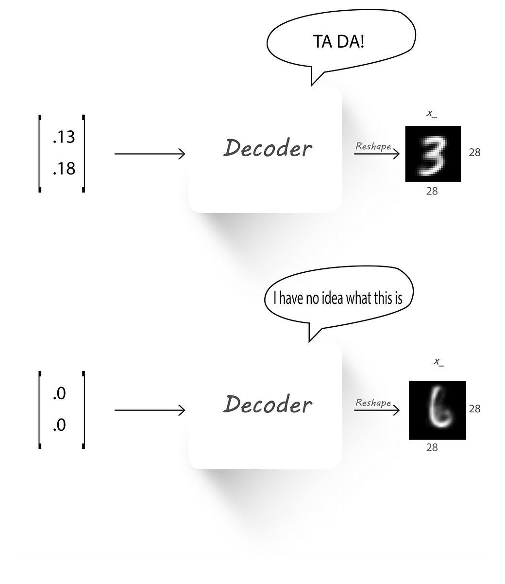
We left off part 1 by passing a value (0, 0) to our trained decoder (which has 2 neurons at the input) and finding its output. It looked blurry and didn’t represent a clear digit leaving us
with the conclusion that the output of the encoder h (also known as the latent code) was not distributed evenly in a particular space.
So, our main aim in this part will be to force the encoder output to match a given prior distribution, this required distribution can be a normal (Gaussian) distribution, uniform distribution,
gamma distribution… . This should then cause the latent code (encoder output) to be evenly distributed over the given prior distribution, which would allow our decoder to learn a mapping from the prior to a data distribution (distribution of MNIST images in
our case).
If you understood absolutely nothing from the above paragraph.
Let’s say you’re in college and have opted to take up Machine Learning (I couldn’t think of another course :p) as one of your courses.
Now, if the course instructor doesn’t provide a syllabus guide or a reference book then, what will you study for your finals? (assume your classes weren’t helpful).
You could be asked questions from any subfield of ML, what would you do? Makeup stuff with what you know??
This is what happens if we don’t constrain our encoder output to follow some distribution, the decoder cannot learn a mapping from any number
to an image.
But, if you are given a proper syllabus guide then, you can just go through the materials before the exam and you’ll have an idea of what to
expect.
Similarly, if we force the encoder output to follow a known distribution like a Gaussian, then it can learn to spread the latent code to cover
the entire distribution and learn mappings without any gap.
Good or Bad?
We now know that an autoencoder has two parts, each performing a completely opposite task.
Two people of similar nature can never get alone, it takes two opposites to harmonize.
— Ram Mohan
The encoder which is used to get a latent code (encoder output) from the input with the constraint that the dimension of the latent code should be less than the input dimension and
secondly, the decoder that takes in this latent code and tries to reconstruct the original image.
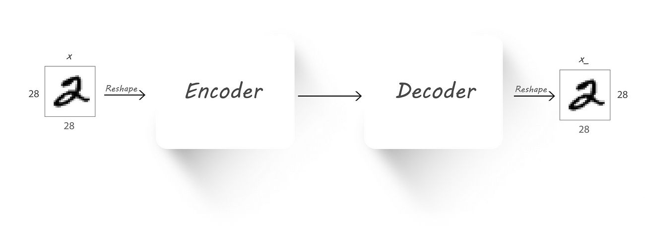
Autoencoder Block diagram
Let’s see how the encoder output was distributed when we previously implemented our autoencoder (checkout part
1):
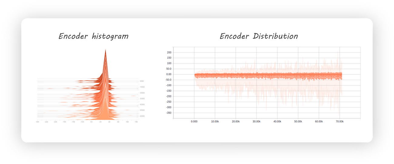
Encoder histogram and distribution
From the distribution graph (which is towards the right) we can clearly see that our encoder’s output distribution is all over the place. Initially, it appears as though the distribution
is centred at 0 with most of the values being negative. At later stages during training the negative samples are distributed farther away from 0 when compared to the positive ones (also, we might not even get the same distribution if we run the experiment
again). This leads to large amounts of gaps in the encoder distribution which isn’t a good thing if we want to use our decoder as a generative model.
But, why are these gaps a bad thing to have in our encoder distribution?
If we give an input that falls in this gap to a trained decoder then it’ll give weird looking images which don’t represent digits at its output (I know, 3rd time).
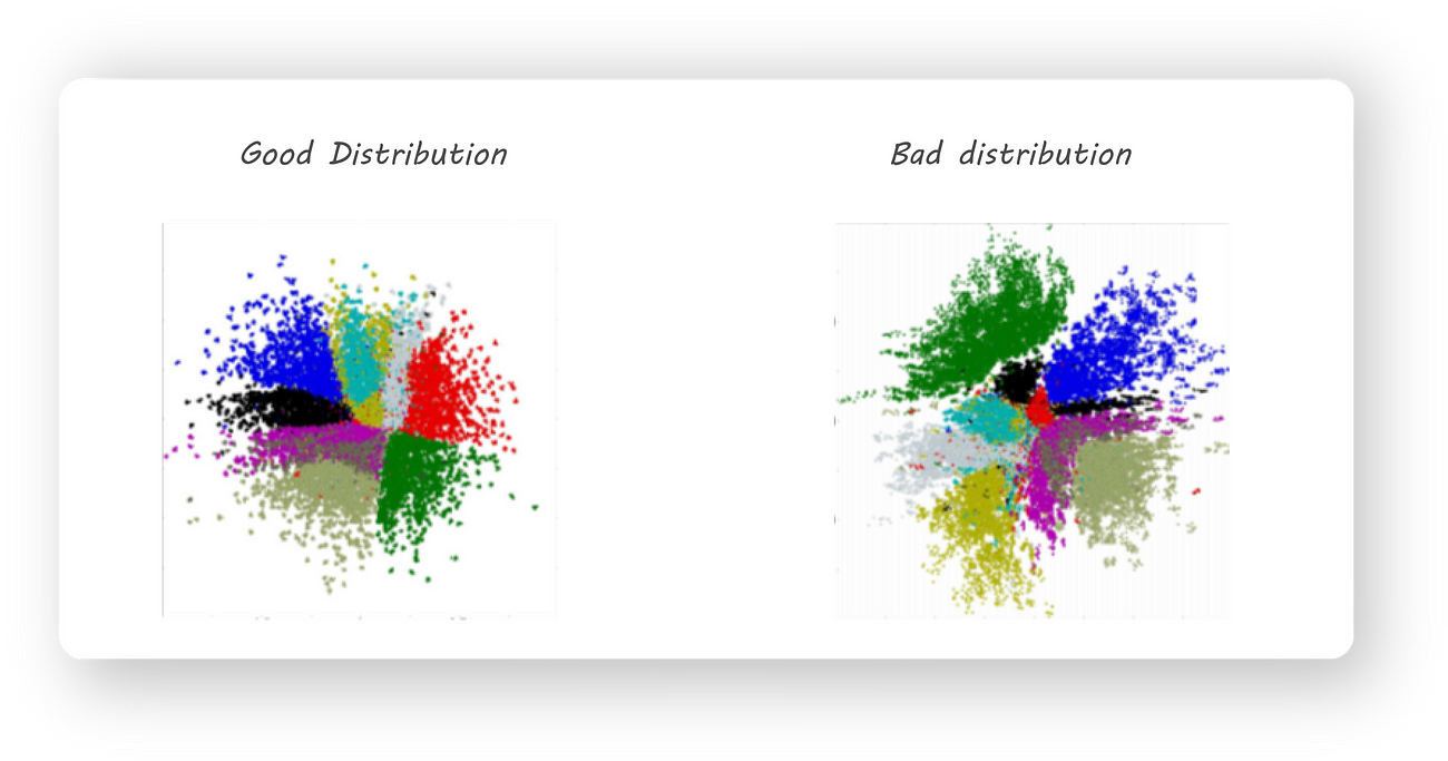
Another important observation that was made is that training an autoencoder gives us latent codes with similar images (for example all 2s or 3s ..) being far from each other in the euclidean
space. This, for example, can cause all the 2s in our dataset to be mapped to different regions in space. We want the latent code to have a meaningful representation by keeping images of similar digits close together. Some thing like this:

A good 2D distribution
Different colored regions represent one class of images, notice how the same colored regions are close to one another.
We now look at Adversarial Autoencoders that can solve some of the above mentioned problems.
An Adversarial autoencoder is quite similar to an autoencoder but the encoder is trained in an adversarial manner to force it to output a required distribution.
Understanding Adversarial Autoencoders (AAEs) requires knowledge of Generative Adversarial Networks (GANs), I have written an article on GANs which can be found here:
GANs
N’ Roses
“This article assumes the reader is familiar with Neural networks and using Tensorflow. If not, we
would request you to…medium.com
If you already know about GANs here’s a quick recap (feel free to skip this section if you remember the next two points):
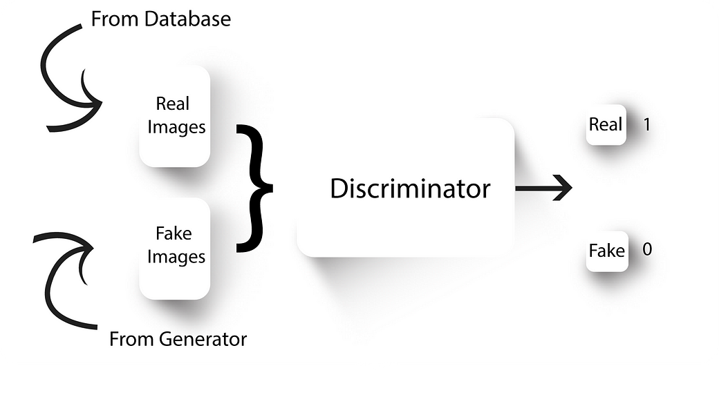
Discriminator
Generator
GANs have two neural nets, a generator and a discriminator.
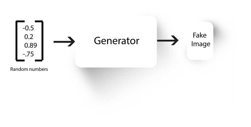
Generator, well generates fake images. We train the discriminator to tell apart real images from our dataset with the fake ones generated by our generator.
The generator initially generates some random noise (because it’s weights will be random). After training our discriminator to discriminate this random noise and real images, we’ll connect
our generator to our discriminator and backprop only through the generator with the constraint that the discriminator output should be 1 (i.e, the discriminator should classify the output of the generator as real images).
We’ll again train our discriminator to now tell apart the new fake images from our generator and the real ones from our database. This is followed by training the generated to generate
better fake looking images.
We’ll continue this process until the generator becomes so good at generating fake images that the discriminator is no longer able to tell real images from fake ones.
At the end, we’ll be left with a generator which can produce real looking fake images given a random set of numbers as its input.
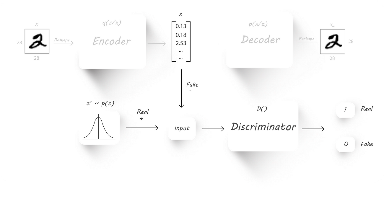
Here’s a block diagram of an Adversarial Autoencoder:
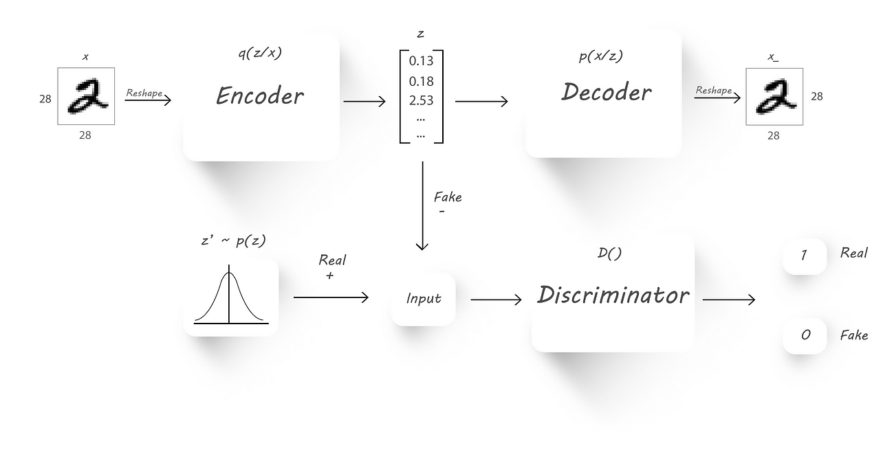
AAE block diagram
x → Input image
q(z/x) → Encoder output given input x
z → Latent code (fake input), z is drawn from q(z/x)
z’ → Real input with the required distribution
p(x/z) →Decoder output given z
D() → Discriminator
x_ →Reconstructed image
Again, our main is to force the encoder to output values which have a given prior distribution (this can be normal, gamma .. distributions). We’ll use the encoder (q(z/x)) as our generator,
the discriminator to tell if the samples are from a prior distribution (p(z)) or from the output of the encoder (z) and the decoder (p(x/z)) to get back the original input image.
To get an understanding of how this architecture could be used to impose a prior distribution on the encoder output, lets have a look at how we go about training an AAE.
Training an AAE has 2 phases:
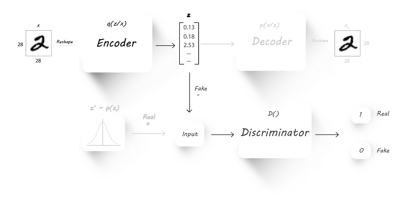
Reconstruction phase:
We’ll train both the encoder and the decoder to minimize the reconstruction loss (mean squared error between the input and the decoder output images, checkout part 1 for more details). Forget
that the discriminator even exists in this phase (I’ve greyed out the parts that aren’t required in this phase).
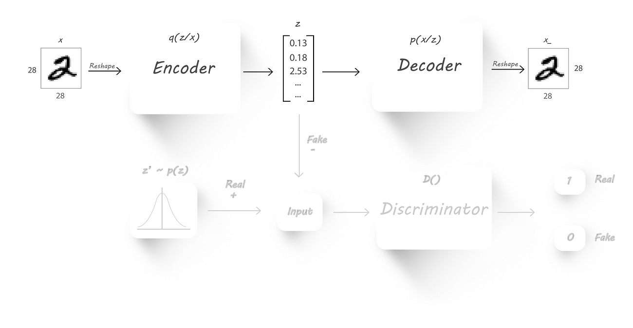
Reconstruction Phase
As usual we’ll pass inputs to the encoder which will give us our latent code, later, we’ll pass this latent code to the decoder to get back the input image. We’ll backprop through both
the encoder and the decoder weights so that reconstruction loss will be reduced.
Regularization phase:
In this phase we’ll have to train the discriminator and the generator (which is nothing but our encoder). Just forget that the decoder exists.
Training the discriminator
First, we train the discriminator to classify the encoder output (z) and some random input(z’, this will have our required distribution). For example, the random input can be normally
distributed with a mean of 0 and standard deviation of 5.
So, the discriminator should give us an output 1 if we pass in random inputs with the desired distribution (real values) and should give us an output 0 (fake values) when we pass in the encoder
output. Intuitively, both the encoder output and the random inputs to the discriminator should have the same size.
The next step will be to force the encoder to output latent code with the desired distribution. To accomplish this we’ll connect the encoder output as the input to the discriminator:
We’ll fix the discriminator weights to whatever they are currently (make them untrainable) and fix the target to 1 at the discriminator output. Later, we pass in images to the encoder and find the discriminator output which is then used to find the loss (cross-entropy
cost function). We’ll backprop only through the encoder weights, which causes the encoder to learn the required distribution and produce output which’ll have that distribution (fixing the discriminator target to 1 should cause the encoder to learn the required
distribution by looking at the discriminator weights).
Now that the theoretical part of out of the way, let’s have a look at how we can implement this using tensorflow.
Here’s the entire code for Part 2 (It’s very similar to what we’ve discussed in Part 1):
Naresh1318/Adversarial_Autoencoder
Adversarial_Autoencoder - A wizard's guide to Adversarial Autoencodersgithub.com
As usual we have our helper
I haven’t changed the encoder and the decoder architectures:
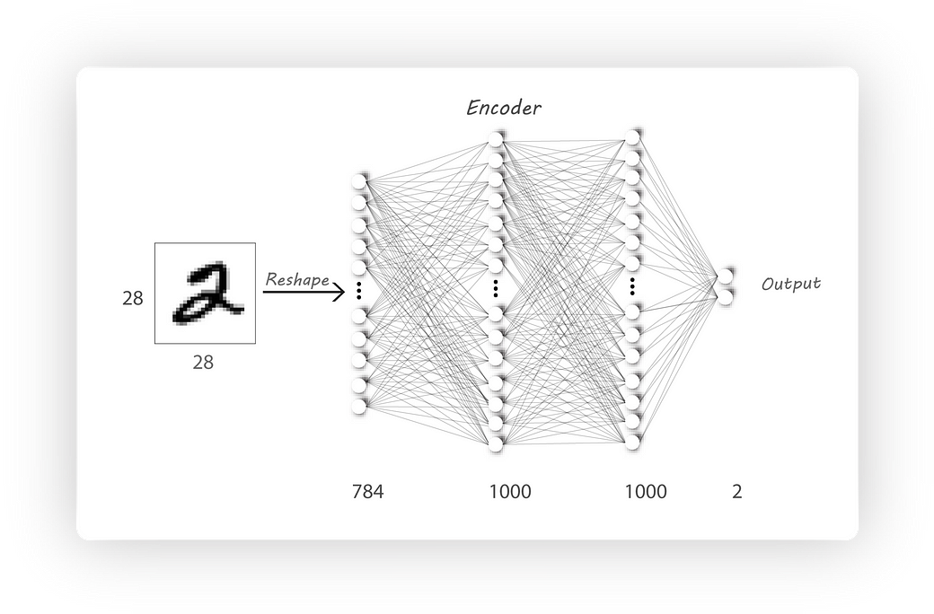
Encoder Architecture
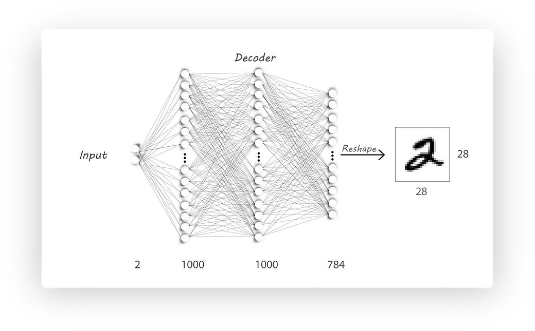
Decoder Architecture
Here’s the discriminator architecture:
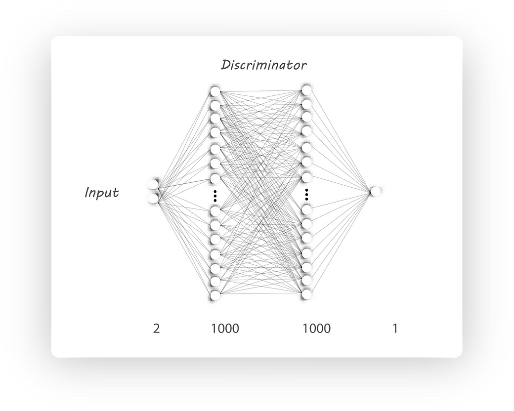
Discriminator Architecture
It’s similar to our encoder architecture, the input shape is
Note that I’ve used the prefixes
defining the dense layers for the encoder, decoder and discriminator respectively. Using these notations help us collect the weights to be trained easily:
We now know that training an AAE has two parts, first being the reconstruction phase (we’ll train our autoencoder to reconstruct the input) and the regularization phase (first the discriminator
is trained followed by the encoder).
We’ll begin the reconstruction phase by connecting our encoder output to the decoder input:
I’ve used
time I call any of our defined architectures as it’ll allow us to share the weights among all function calls (this happens only if
The loss function as usual is the Mean Squared Error (MSE), which we’ve come across in part
1.
Similar to what we did in part 1, the optimizer (which’ll update the weights to reduce the loss[hopefully]) is implemented as follows:
I couldn’t help it :P
That’s it for the reconstruction phase, next we move on to the regularization phase:
We’ll first train the discriminator to distinguish between the real distribution samples and the fake ones from the generator (encoder in this case).
a placeholder which I’ve used to pass in values with the required distribution to the discriminator (this will be our real input).
to the discriminator which’ll give us our discriminator output for fake inputs
Here
we want the same discriminator weights in the second call (if this is not specified, then tensorflow creates new set of randomly initialized weights [but since I’ve used
create the weights it’ll through an error]).
The loss function I’ve used to train the discriminator is:
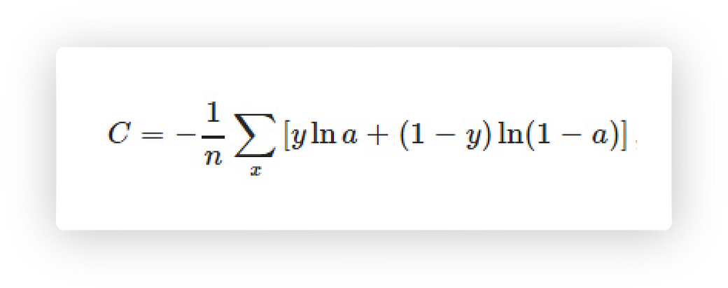
Cross entropy cost
This can easily be implemented in tensorflow as follows:
Next step will be to train the generator (encoder) to output a required distribution. As we have discussed, this requires the discrminator’s target to be set to 1 and the
(the encoder connected to the discriminator [go back and look]). The generator loss is again cross entropy cost function.
To update only the required weights during training we’ll need to pass in all those collected weights to the
under
and the generator (encoder) variables (
We’re almost done, all we have left is to pass our MNIST images as the input and as target along with random numbers of size
The training part might look intimidating, but stare at it for a while you’ll find out that it’s quite intuitive.
The parameters I’ve used during training are as follows:
I trained the model for 300 epochs with required distribution begin a normal (Gaussian) having mean 0 and 5 as it’s standard distribution. Here’s the encoder output and the required distributions
along with their histograms:
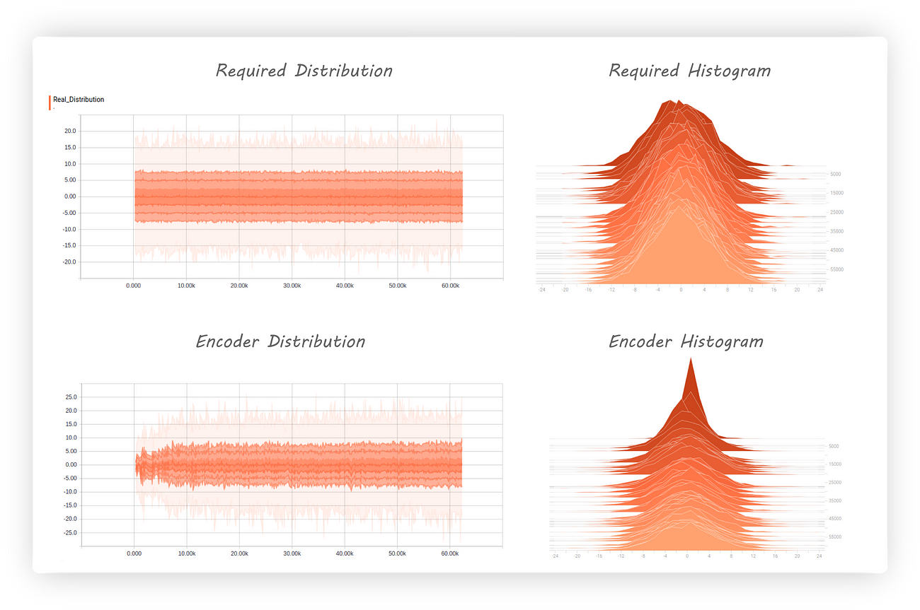
The encoder distribution almost matches the required distribution and the histogram shows us that it’s centred at zero. Great, but what about the discriminator, how well has it fared?
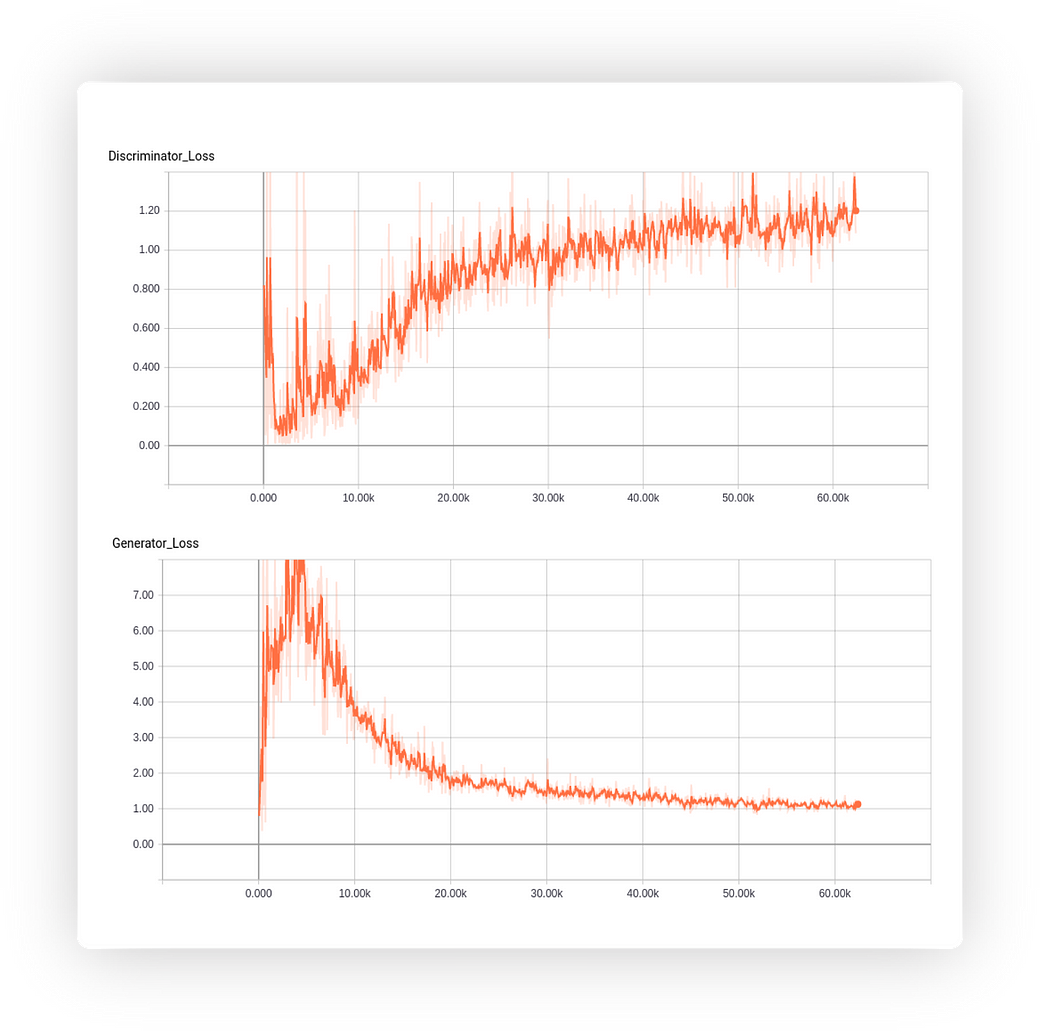
Good news, the discriminator loss is increasing (getting worst) which tells us it’s having a hard time telling apart real and fake inputs.
Lastly, since we have our
values) we can pass in random inputs which fall under the required distribution to our trained decoder and use it as a generator (I know, I was calling encoder as the generator all this while as it was generating fake inputs to the discriminator, but since
the decoder has learn’t to map these fake inputs to get digits at its output we can call our decoder as a generator). I’ve passed values from (-10, -10) to (10, 10) at regular intervals to the decoder and stored its outputs here’s how the digits have been
distributed:
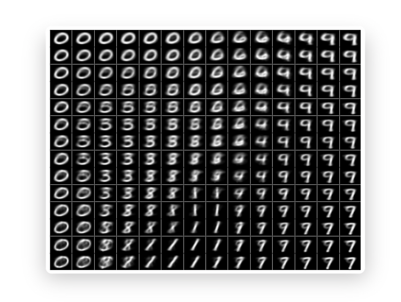
The above figure shows a clear clustering of digits and their transition as we explore values that the decoder is trained at. An AAE has cause the gaps in the encoder output distribution
to get closer which allowed us to use the decoder as a generator.
That’s it!. We’ll focus on how we can use AAE to separate image style from it’s content in the next part. It’s quite easy to implement it since we are done most of the relatively tough parts.
Hope you liked this article on AAEs. I would openly encourage any criticism or suggestions to improve my work.
原文地址:https://medium.com/towards-data-science/a-wizards-guide-to-adversarial-autoencoders-part-2-exploring-latent-space-with-adversarial-2d53a6f8a4f9
wizard’s guide to Autoencoders: Part 1, if you haven’t read it but are familiar with the basics of autoencoders then continue on. You’ll need to know a little bit about probability theory which can
be found here.”
Part 1: Autoencoder?
We left off part 1 by passing a value (0, 0) to our trained decoder (which has 2 neurons at the input) and finding its output. It looked blurry and didn’t represent a clear digit leaving us
with the conclusion that the output of the encoder h (also known as the latent code) was not distributed evenly in a particular space.
So, our main aim in this part will be to force the encoder output to match a given prior distribution, this required distribution can be a normal (Gaussian) distribution, uniform distribution,
gamma distribution… . This should then cause the latent code (encoder output) to be evenly distributed over the given prior distribution, which would allow our decoder to learn a mapping from the prior to a data distribution (distribution of MNIST images in
our case).
If you understood absolutely nothing from the above paragraph.
Let’s say you’re in college and have opted to take up Machine Learning (I couldn’t think of another course :p) as one of your courses.
Now, if the course instructor doesn’t provide a syllabus guide or a reference book then, what will you study for your finals? (assume your classes weren’t helpful).
You could be asked questions from any subfield of ML, what would you do? Makeup stuff with what you know??
This is what happens if we don’t constrain our encoder output to follow some distribution, the decoder cannot learn a mapping from any number
to an image.
But, if you are given a proper syllabus guide then, you can just go through the materials before the exam and you’ll have an idea of what to
expect.
Similarly, if we force the encoder output to follow a known distribution like a Gaussian, then it can learn to spread the latent code to cover
the entire distribution and learn mappings without any gap.
Good or Bad?
We now know that an autoencoder has two parts, each performing a completely opposite task.
Two people of similar nature can never get alone, it takes two opposites to harmonize.
— Ram Mohan
The encoder which is used to get a latent code (encoder output) from the input with the constraint that the dimension of the latent code should be less than the input dimension and
secondly, the decoder that takes in this latent code and tries to reconstruct the original image.
Autoencoder Block diagram
Let’s see how the encoder output was distributed when we previously implemented our autoencoder (checkout part
1):
Encoder histogram and distribution
From the distribution graph (which is towards the right) we can clearly see that our encoder’s output distribution is all over the place. Initially, it appears as though the distribution
is centred at 0 with most of the values being negative. At later stages during training the negative samples are distributed farther away from 0 when compared to the positive ones (also, we might not even get the same distribution if we run the experiment
again). This leads to large amounts of gaps in the encoder distribution which isn’t a good thing if we want to use our decoder as a generative model.
But, why are these gaps a bad thing to have in our encoder distribution?
If we give an input that falls in this gap to a trained decoder then it’ll give weird looking images which don’t represent digits at its output (I know, 3rd time).
Another important observation that was made is that training an autoencoder gives us latent codes with similar images (for example all 2s or 3s ..) being far from each other in the euclidean
space. This, for example, can cause all the 2s in our dataset to be mapped to different regions in space. We want the latent code to have a meaningful representation by keeping images of similar digits close together. Some thing like this:
A good 2D distribution
Different colored regions represent one class of images, notice how the same colored regions are close to one another.
We now look at Adversarial Autoencoders that can solve some of the above mentioned problems.
An Adversarial autoencoder is quite similar to an autoencoder but the encoder is trained in an adversarial manner to force it to output a required distribution.
Understanding Adversarial Autoencoders (AAEs) requires knowledge of Generative Adversarial Networks (GANs), I have written an article on GANs which can be found here:
GANs
N’ Roses
“This article assumes the reader is familiar with Neural networks and using Tensorflow. If not, we
would request you to…medium.com
If you already know about GANs here’s a quick recap (feel free to skip this section if you remember the next two points):
Discriminator
Generator
GANs have two neural nets, a generator and a discriminator.
Generator, well generates fake images. We train the discriminator to tell apart real images from our dataset with the fake ones generated by our generator.
The generator initially generates some random noise (because it’s weights will be random). After training our discriminator to discriminate this random noise and real images, we’ll connect
our generator to our discriminator and backprop only through the generator with the constraint that the discriminator output should be 1 (i.e, the discriminator should classify the output of the generator as real images).
We’ll again train our discriminator to now tell apart the new fake images from our generator and the real ones from our database. This is followed by training the generated to generate
better fake looking images.
We’ll continue this process until the generator becomes so good at generating fake images that the discriminator is no longer able to tell real images from fake ones.
At the end, we’ll be left with a generator which can produce real looking fake images given a random set of numbers as its input.
Here’s a block diagram of an Adversarial Autoencoder:
AAE block diagram
x → Input image
q(z/x) → Encoder output given input x
z → Latent code (fake input), z is drawn from q(z/x)
z’ → Real input with the required distribution
p(x/z) →Decoder output given z
D() → Discriminator
x_ →Reconstructed image
Again, our main is to force the encoder to output values which have a given prior distribution (this can be normal, gamma .. distributions). We’ll use the encoder (q(z/x)) as our generator,
the discriminator to tell if the samples are from a prior distribution (p(z)) or from the output of the encoder (z) and the decoder (p(x/z)) to get back the original input image.
To get an understanding of how this architecture could be used to impose a prior distribution on the encoder output, lets have a look at how we go about training an AAE.
Training an AAE has 2 phases:
Reconstruction phase:
We’ll train both the encoder and the decoder to minimize the reconstruction loss (mean squared error between the input and the decoder output images, checkout part 1 for more details). Forget
that the discriminator even exists in this phase (I’ve greyed out the parts that aren’t required in this phase).
Reconstruction Phase
As usual we’ll pass inputs to the encoder which will give us our latent code, later, we’ll pass this latent code to the decoder to get back the input image. We’ll backprop through both
the encoder and the decoder weights so that reconstruction loss will be reduced.
Regularization phase:
In this phase we’ll have to train the discriminator and the generator (which is nothing but our encoder). Just forget that the decoder exists.
Training the discriminator
First, we train the discriminator to classify the encoder output (z) and some random input(z’, this will have our required distribution). For example, the random input can be normally
distributed with a mean of 0 and standard deviation of 5.
So, the discriminator should give us an output 1 if we pass in random inputs with the desired distribution (real values) and should give us an output 0 (fake values) when we pass in the encoder
output. Intuitively, both the encoder output and the random inputs to the discriminator should have the same size.
The next step will be to force the encoder to output latent code with the desired distribution. To accomplish this we’ll connect the encoder output as the input to the discriminator:
We’ll fix the discriminator weights to whatever they are currently (make them untrainable) and fix the target to 1 at the discriminator output. Later, we pass in images to the encoder and find the discriminator output which is then used to find the loss (cross-entropy
cost function). We’ll backprop only through the encoder weights, which causes the encoder to learn the required distribution and produce output which’ll have that distribution (fixing the discriminator target to 1 should cause the encoder to learn the required
distribution by looking at the discriminator weights).
Now that the theoretical part of out of the way, let’s have a look at how we can implement this using tensorflow.
Here’s the entire code for Part 2 (It’s very similar to what we’ve discussed in Part 1):
Naresh1318/Adversarial_Autoencoder
Adversarial_Autoencoder - A wizard's guide to Adversarial Autoencodersgithub.com
As usual we have our helper
dense():
I haven’t changed the encoder and the decoder architectures:
Encoder Architecture
Decoder Architecture
Here’s the discriminator architecture:
Discriminator Architecture
It’s similar to our encoder architecture, the input shape is
z_dim(
batch_size,
z_dim
actually) and the output has a shape of 1 (
batch_size, 1).
Note that I’ve used the prefixes
e_,
d_and
dc_while
defining the dense layers for the encoder, decoder and discriminator respectively. Using these notations help us collect the weights to be trained easily:
We now know that training an AAE has two parts, first being the reconstruction phase (we’ll train our autoencoder to reconstruct the input) and the regularization phase (first the discriminator
is trained followed by the encoder).
We’ll begin the reconstruction phase by connecting our encoder output to the decoder input:
I’ve used
tf.variable_scope(tf.get_variable_scope())each
time I call any of our defined architectures as it’ll allow us to share the weights among all function calls (this happens only if
reuse=True).
The loss function as usual is the Mean Squared Error (MSE), which we’ve come across in part
1.
Similar to what we did in part 1, the optimizer (which’ll update the weights to reduce the loss[hopefully]) is implemented as follows:
I couldn’t help it :P
That’s it for the reconstruction phase, next we move on to the regularization phase:
We’ll first train the discriminator to distinguish between the real distribution samples and the fake ones from the generator (encoder in this case).
real_distributionis
a placeholder which I’ve used to pass in values with the required distribution to the discriminator (this will be our real input).
encoder_outputis connected
to the discriminator which’ll give us our discriminator output for fake inputs
d_fake.
Here
reuse=Truesince
we want the same discriminator weights in the second call (if this is not specified, then tensorflow creates new set of randomly initialized weights [but since I’ve used
get_variable()to
create the weights it’ll through an error]).
The loss function I’ve used to train the discriminator is:
Cross entropy cost
This can easily be implemented in tensorflow as follows:
Next step will be to train the generator (encoder) to output a required distribution. As we have discussed, this requires the discrminator’s target to be set to 1 and the
d_fakevariable
(the encoder connected to the discriminator [go back and look]). The generator loss is again cross entropy cost function.
To update only the required weights during training we’ll need to pass in all those collected weights to the
var_listparameter
under
minimize(). So, I’ve passed in the discriminator variables (
dc_var)
and the generator (encoder) variables (
en_var) during their training phases.
We’re almost done, all we have left is to pass our MNIST images as the input and as target along with random numbers of size
batch_size,
z_dim
as inputs to the discriminator (this will form the required distribution).
The training part might look intimidating, but stare at it for a while you’ll find out that it’s quite intuitive.
The parameters I’ve used during training are as follows:
I trained the model for 300 epochs with required distribution begin a normal (Gaussian) having mean 0 and 5 as it’s standard distribution. Here’s the encoder output and the required distributions
along with their histograms:
The encoder distribution almost matches the required distribution and the histogram shows us that it’s centred at zero. Great, but what about the discriminator, how well has it fared?
Good news, the discriminator loss is increasing (getting worst) which tells us it’s having a hard time telling apart real and fake inputs.
Lastly, since we have our
z_dim=2(2D
values) we can pass in random inputs which fall under the required distribution to our trained decoder and use it as a generator (I know, I was calling encoder as the generator all this while as it was generating fake inputs to the discriminator, but since
the decoder has learn’t to map these fake inputs to get digits at its output we can call our decoder as a generator). I’ve passed values from (-10, -10) to (10, 10) at regular intervals to the decoder and stored its outputs here’s how the digits have been
distributed:
The above figure shows a clear clustering of digits and their transition as we explore values that the decoder is trained at. An AAE has cause the gaps in the encoder output distribution
to get closer which allowed us to use the decoder as a generator.
That’s it!. We’ll focus on how we can use AAE to separate image style from it’s content in the next part. It’s quite easy to implement it since we are done most of the relatively tough parts.
Hope you liked this article on AAEs. I would openly encourage any criticism or suggestions to improve my work.
原文地址:https://medium.com/towards-data-science/a-wizards-guide-to-adversarial-autoencoders-part-2-exploring-latent-space-with-adversarial-2d53a6f8a4f9

相关文章推荐
- A wizard’s guide to Adversarial Autoencoders: Part 1, Autoencoder?
- A wizard’s guide to Adversarial Autoencoders: Part 3, Disentanglement of style and content.
- Visual guide to Windows Live ID authentication with SharePoint 2010 - part 1
- Harder Monsters and More Levels: How To Make A Simple iPhone Game with Cocos2D Part 3
- Stanford UFLDL教程 Exercise:Learning color features with Sparse Autoencoders
- A Beginner's Guide To Understanding Convolutional Neural Networks Part 2
- Image-to-Image Translation with Conditional Adversarial Networks
- How to make a combo box with fulltext search autocomplete support?
- A complete guide to using Keras as part of a TensorFlow workflow: tutorial
- An introduction to Generative Adversarial Networks (with code in TensorFlow)
- Auto Complete Tutorial for iOS: How To Auto Complete With Custom Values
- How to setup multiple sites hosted on your Mac with OSX 10.8 + (MAMP Part 5)
- A Complete Guide to Usage of ‘usermod’ command– 15 Practical Examples with Screenshots
- A Guide to Undefined Behavior in C and C++, Part 1
- Occlusion-free Face Alignment: Deep Regression Networks Coupled with De-corrupt AutoEncoders
- 卷积神经Extracting and Composing Robust Features with Denoising Autoencoders
- How to train models of Object Detection with Discriminatively Trained Part Based Models
- iphone游戏开发-Collisions and Collectables: How To Make a Tile Based Game with Cocos2D Part 2
- tablespace occuped with autoextent managment and tempfile
- How to Get Started with JMeter: Part 3 – Reports & Performance Metrics Best Practices