【机器学习】回归分析、过拟合、分类
2017-10-23 09:53
465 查看
一、Linear Regression
线性回归是相对简单的一种,表达式如下
View Code
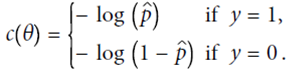
五、Logistic Regression(可用作分类)
[b]
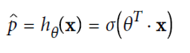
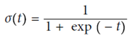
(使用sigmod函数,y在(0,1)之间)
定义cost function,由于p在(0,1)之间,故最前面加一个符号,保证代价始终为正的。p值越大,整体cost越小,预测的越对
即
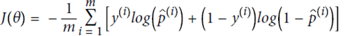
不存在解析解,故用偏导数计算
以Iris花的种类划分为例

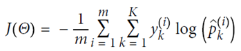
六、Softmax Regression
可以用做多分类

使用交叉熵
线性回归是相对简单的一种,表达式如下
from sklearn.base import clone
sgd_reg = SGDRegressor(n_iter=1, warm_start=True, penalty=None,
learning_rate="constant", eta0=0.0005)
minimum_val_error = float("inf")
best_epoch = None
best_model = None
for epoch in range(1000):
sgd_reg.fit(X_train_poly_scaled, y_train) # continues where it left off
y_val_predict = sgd_reg.predict(X_val_poly_scaled)
val_error = mean_squared_error(y_val_predict, y_val)
if val_error < minimum_val_error:
minimum_val_error = val_error
best_epoch = epoch
best_model = clone(sgd_reg)
View Code
五、Logistic Regression(可用作分类)
[b]
(使用sigmod函数,y在(0,1)之间)
定义cost function,由于p在(0,1)之间,故最前面加一个符号,保证代价始终为正的。p值越大,整体cost越小,预测的越对
即
不存在解析解,故用偏导数计算
以Iris花的种类划分为例
import matplotlib.pyplot as plt
from sklearn import datasets
iris = datasets.load_iris()
print(list(iris.keys()))
# ['DESCR', 'data', 'target', 'target_names', 'feature_names']
X = iris["data"][:, 3:] # petal width
y = (iris["target"] == 2).astype(np.int) # 1 if Iris-Virginica, else 0

from sklearn.linear_model import LogisticRegression
log_reg = LogisticRegression()
log_reg.fit(X, y)
X_new = np.linspace(0, 3, 1000).reshape(-1, 1)
# estimated probabilities for flowers with petal widths varying from 0 to 3 cm:
y_proba = log_reg.predict_proba(X_new)

plt.plot(X_new, y_proba[:, 1], "g-", label="Iris-Virginica")
plt.plot(X_new, y_proba[:, 0], "b--", label="Not Iris-Virginica")
plt.show()
# + more Matplotlib code to make the image look pretty
六、Softmax Regression
可以用做多分类
使用交叉熵
X = iris["data"][:, (2, 3)] # petal length, petal width
y = iris["target"]
softmax_reg = LogisticRegression(multi_class="multinomial",solver="lbfgs", C=10)
softmax_reg.fit(X, y)

print(softmax_reg.predict([[5, 2]]))
# array([2])
print(softmax_reg.predict_proba([[5, 2]]))
# array([[ 6.33134078e-07, 5.75276067e-02, 9.42471760e-01]])

相关文章推荐
- 【机器学习入门】Andrew NG《Machine Learning》课程笔记之四:分类、逻辑回归和过拟合
- 回归,分类与聚类:三个方向分析机器学习
- 斯坦福机器学习-第三周(分类,逻辑回归,过度拟合及解决方法)
- 什么叫“回归”——“回归”名词的由来&&回归与拟合、分类的区别 && 回归分析
- 什么叫“回归”——“回归”名词的由来&&回归与拟合、分类的区别 && 回归分析
- 机器学习回归算法—岭回归及案例分析
- CART分类回归树分析与python实现
- 机器学习---之逻辑回归,贝耶斯分类与极大似然估计的联系
- CART决策树(分类回归树)分析及应用建模
- 机器学习-分类和逻辑回归
- Python机器学习(二):Logistic回归建模分类实例——信用卡欺诈监测(上)
- 【Stanford Machine Learning Open Course】8. 过拟合问题解决以及在回归问题和分类问题上的应用
- Python数据分析与机器学习-新闻分类任务
- Coursera机器学习 Week3:逻辑回归、Decision Boundary、过拟合
- 机器学习2——分类和逻辑回归Classification and logistic regression(牛顿法待研究)
- 机器学习:决策树cart算法在分类与回归的应用(下)
- 机器学习:以二元决策树为基学习器实现随机森林算法的回归分析
- 逻辑斯底回归的特征、多分类问题及过拟合问题
- [机器学习]逻辑回归,Logistic regression |分类,Classification
- 逻辑回归(Logistic Regression, LR)又称为逻辑回归分析,是分类和预测算法中的一种。通过历史数据的表现对未来结果发生的概率进行预测。例如,我们可以将购买的概率设置为因变量,将用户的