Coursera-Deep Learning Specialization 课程之(一):Neural Networks and Deep Learning-weak2编程作业
2017-10-17 16:16
676 查看
一 Python Basics with numpy (optional)
学习目标:①使用logistic regression
②学习如何最小化代价函数cost function
③理解通过代价函数的导数来更新参数**
1 - Building basic functions with numpy
1.1 - sigmoid function, np.exp()
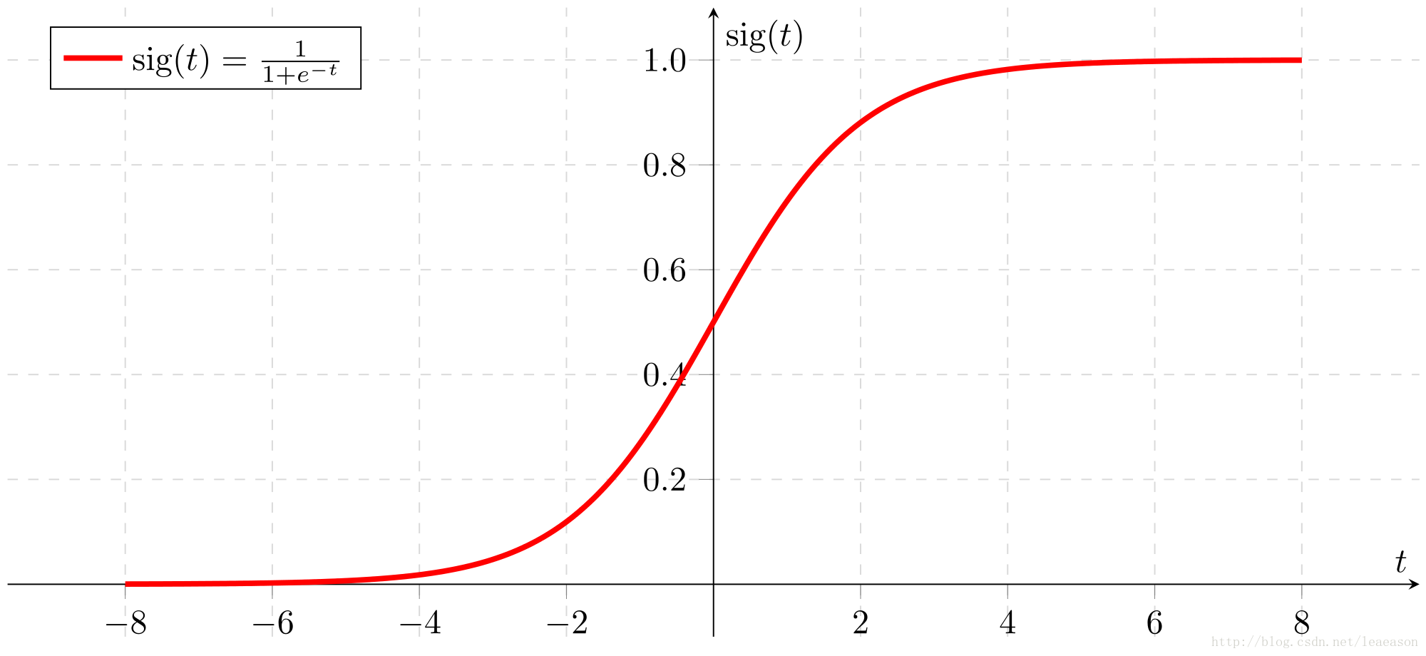
# GRADED FUNCTION: basic_sigmoid

import math

def basic_sigmoid(x):
"""
Compute sigmoid of x.
Arguments:
x -- A scalar
Return:
s -- sigmoid(x)
"""
### START CODE HERE ### (≈ 1 line of code)
s = 1/(1+math.exp(-x))
### END CODE HERE ###
return s
basic_sigmoid(3)
0.9525741268224334
# GRADED FUNCTION: sigmoid
import numpy as np # this means you can access numpy functions by writing np.function() instead of numpy.function()
def sigmoid(x):
"""
Compute the sigmoid of x
Arguments:
x -- A scalar or numpy array of any size
Return:
s -- sigmoid(x)
"""
### START CODE HERE ### (≈ 1 line of code)
s = 1/(1+np.exp(-x))
### END CODE HERE ###
return s
1.2 - Sigmoid gradient
# GRADED FUNCTION: sigmoid_derivative
def sigmoid_derivative(x):
"""
Compute the gradient (also called the slope or derivative) of the sigmoid function with respect to its input x.
You can store the output of the sigmoid function into variables and then use it to calculate the gradient.
Arguments:
x -- A scalar or numpy array
Return:
ds -- Your computed gradient.
"""
### START CODE HERE ### (≈ 2 lines of code)
s = sigmoid(x)
ds = s*(1-s)
### END CODE HERE ###
return ds
1.3 - Reshaping arrays
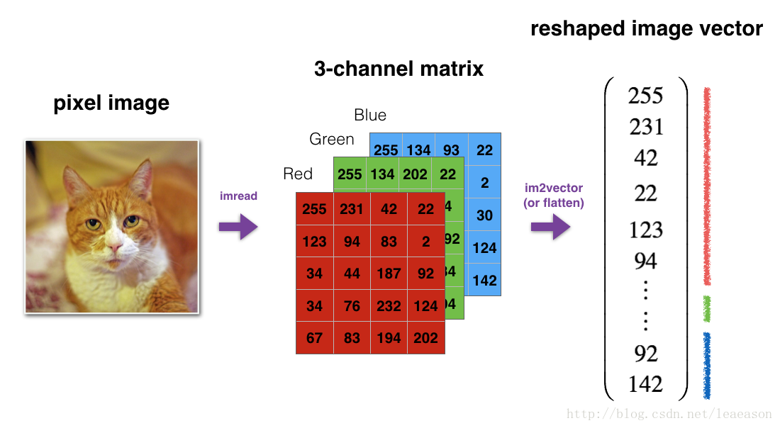
# GRADED FUNCTION: image2vector
def image2vector(image):
"""
Argument:
image -- a numpy array of shape (length, height, depth)
Returns:
v -- a vector of shape (length*height*depth, 1)
"""
### START CODE HERE ### (≈ 1 line of code)
v = image.reshape(image.shape[0]*image.shape[1]*image.shape[2],1)
### END CODE HERE ###
return v
# This is a 3 by 3 by 2 array, typically images will be (num_px_x, num_px_y,3) where 3 represents the RGB values
image = np.array([[[ 0.67826139,  0.29380381],
[ 0.90714982,  0.52835647],
[ 0.4215251 ,  0.45017551]],
[[ 0.92814219,  0.96677647],
[ 0.85304703,  0.52351845],
[ 0.19981397,  0.27417313]],
[[ 0.60659855,  0.00533165],
[ 0.10820313,  0.49978937],
[ 0.34144279,  0.94630077]]])
print ("image2vector(image) = " + str(image2vector(image)))
1.4 - Normalizing rows
# GRADED FUNCTION: normalizeRows
def normalizeRows(x):
"""
Implement a function that normalizes each row of the matrix x (to have unit length).
Argument:
x -- A numpy matrix of shape (n, m)
Returns:
x -- The normalized (by row) numpy matrix. You are allowed to modify x.
"""
### START CODE HERE ### (≈ 2 lines of code)
# Compute x_norm as the norm 2 of x. Use np.linalg.norm(..., ord = 2, axis = ..., keepdims = True)
x_norm = np.linalg.norm(x,ord=2,axis=1,keepdims=True)
# Divide x by its norm.
x = x/x_norm
### END CODE HERE ###
return x
1.5 - Broadcasting and the softmax function
# GRADED FUNCTION: softmax
def softmax(x):
"""Calculates the softmax for each row of the input x.
Your code should work for a row vector and also for matrices of shape (n, m).
Argument:
x -- A numpy matrix of shape (n,m)
Returns:
s -- A numpy matrix equal to the softmax of x, of shape (n,m)
"""
### START CODE HERE ### (≈ 3 lines of code)
# Apply exp() element-wise to x. Use np.exp(...).
x_exp = np.exp(x)
# Create a vector x_sum that sums each row of x_exp. Use np.sum(..., axis = 1, keepdims = True).
x_sum = np.sum(x_exp,axis=1,keepdims=True)
# Compute softmax(x) by dividing x_exp by x_sum. It should automatically use numpy broadcasting.
s = x_exp/x_sum
### END CODE HERE ###
return s
2 Vectorization
2.1 Implement the L1 and L2 loss functions
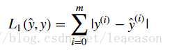
# GRADED FUNCTION: L1
def L1(yhat, y):
"""
Arguments:
yhat -- vector of size m (predicted labels)
y -- vector of size m (true labels)
Returns:
loss -- the value of the L1 loss function defined above
"""
### START CODE HERE ### (≈ 1 line of code)
loss = np.sum(abs(y-yhat))
### END CODE HERE ###
return loss
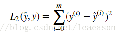
# GRADED FUNCTION: L2
def L2(yhat, y):
"""
Arguments:
yhat -- vector of size m (predicted labels)
y -- vector of size m (true labels)
Returns:
loss -- the value of the L2 loss function defined above
"""
### START CODE HERE ### (≈ 1 line of code)
loss = np.dot(y-yhat,y-yhat)
### END CODE HERE ###
return loss
二 Logistic Regression with a Neural Network mindset
1 - Packages
import numpy as np
import matplotlib.pyplot as plt
import h5py
import scipy
from PIL import Image
from scipy import ndimage
from lr_utils import load_dataset
%matplotlib inline
2 - Overview of the Problem set
# Loading the data (cat/non-cat)
train_set_x_orig, train_set_y, test_set_x_orig, test_set_y, classes = load_dataset()
# Example of a picture
index = 25
plt.imshow(train_set_x_orig[index])
print ("y = " + str(train_set_y[:, index]) + ", it's a '" + classes[np.squeeze(train_set_y[:, index])].decode("utf-8") +  "' picture.")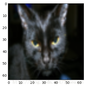
### START CODE HERE ### (≈ 3 lines of code)
m_train = 209
m_test = 50
num_px = 64
### END CODE HERE ###
print ("Number of training examples: m_train = " + str(m_train))
print ("Number of testing examples: m_test = " + str(m_test))
print ("Height/Width of each image: num_px = " + str(num_px))
print ("Each image is of size: (" + str(num_px) + ", " + str(num_px) + ", 3)")
print ("train_set_x shape: " + str(train_set_x_orig.shape))
print ("train_set_y shape: " + str(train_set_y.shape))
print ("test_set_x shape: " + str(test_set_x_orig.shape))
print ("test_set_y shape: " + str(test_set_y.shape))
# Reshape the training and test examples
### START CODE HERE ### (≈ 2 lines of code)
train_set_x_flatten = train_set_x_orig.reshape(train_set_x_orig.shape[0],-1).T
test_set_x_flatten = test_set_x_orig.reshape(test_set_x_orig.shape[0],-1).T
### END CODE HERE ###
print ("train_set_x_flatten shape: " + str(train_set_x_flatten.shape))
print ("train_set_y shape: " + str(train_set_y.shape))
print ("test_set_x_flatten shape: " + str(test_set_x_flatten.shape))
print ("test_set_y shape: " + str(test_set_y.shape))
print ("sanity check after reshaping: " + str(train_set_x_flatten[0:5,0]))3 - General Architecture of the learning algorithm
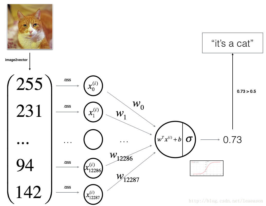
4 - Building the parts of our algorithm
4.1 - Helper functions
# GRADED FUNCTION: sigmoid
def sigmoid(z):
"""
Compute the sigmoid of z
Arguments:
z -- A scalar or numpy array of any size.
Return:
s -- sigmoid(z)
"""
### START CODE HERE ### (≈ 1 line of code)
s = 1/(1+np.exp(-z))
### END CODE HERE ###
return s
4.2 - Initializing parameters
# GRADED FUNCTION: initialize_with_zeros
def initialize_with_zeros(dim):
"""
This function creates a vector of zeros of shape (dim, 1) for w and initializes b to 0.
Argument:
dim -- size of the w vector we want (or number of parameters in this case)
Returns:
w -- initialized vector of shape (dim, 1)
b -- initialized scalar (corresponds to the bias)
"""
### START CODE HERE ### (≈ 1 line of code)
w = np.zeros((dim,1))
b = 0
### END CODE HERE ###
assert(w.shape == (dim, 1))
assert(isinstance(b, float) or isinstance(b, int))
return w, b
4.3 - Forward and Backward propagation
def propagate(w, b, X, Y):
"""
Implement the cost function and its gradient for the propagation explained above
Arguments:
w -- weights, a numpy array of size (num_px * num_px * 3, 1)
b -- bias, a scalar
X -- data of size (num_px * num_px * 3, number of examples)
Y -- true "label" vector (containing 0 if non-cat, 1 if cat) of size (1, number of examples)
Return:
cost -- negative log-likelihood cost for logistic regression
dw -- gradient of the loss with respect to w, thus same shape as w
db -- gradient of the loss with respect to b, thus same shape as b
Tips:
- Write your code step by step for the propagation. np.log(), np.dot()
"""
m = X.shape[1]
# FORWARD PROPAGATION (FROM X TO COST)
### START CODE HERE ### (≈ 2 lines of code)
A = sigmoid(np.dot(w.T,X)+b)                                    # compute activation
cost = -1/m*np.sum(Y*np.log(A)+(1-Y)*np.log(1-A))                               # compute cost
### END CODE HERE ###
# BACKWARD PROPAGATION (TO FIND GRAD)
### START CODE HERE ### (≈ 2 lines of code)
dw = 1/m*np.dot(X,(A-Y).T)
db = 1/m*np.sum(A-Y)
### END CODE HERE ###
assert(dw.shape == w.shape)
assert(db.dtype == float)
cost = np.squeeze(cost)
assert(cost.shape == ())
grads = {"dw": dw,
"db": db}
return grads, cost
d) Optimization
GRADED FUNCTION: optimize
def optimize(w, b, X, Y, num_iterations, learning_rate, print_cost = False):“””
This function optimizes w and b by running a gradient descent algorithm
Arguments:
w -- weights, a numpy array of size (num_px * num_px * 3, 1)
b -- bias, a scalar
X -- data of shape (num_px * num_px * 3, number of examples)
Y -- true "label" vector (containing 0 if non-cat, 1 if cat), of shape (1, number of examples)
num_iterations -- number of iterations of the optimization loop
learning_rate -- learning rate of the gradient descent update rule
print_cost -- True to print the loss every 100 steps
Returns:
params -- dictionary containing the weights w and bias b
grads -- dictionary containing the gradients of the weights and bias with respect to the cost function
costs -- list of all the costs computed during the optimization, this will be used to plot the learning curve.
Tips:
You basically need to write down two steps and iterate through them:
1) Calculate the cost and the gradient for the current parameters. Use propagate().
2) Update the parameters using gradient descent rule for w and b.
"""
costs = []
for i in range(num_iterations):
# Cost and gradient calculation (≈ 1-4 lines of code)
### START CODE HERE ###
grads, cost = propagate(w, b, X, Y)
### END CODE HERE ###
# Retrieve derivatives from grads
dw = grads["dw"]
db = grads["db"]

# update rule (≈ 2 lines of code)
### START CODE HERE ###
w = w-learning_rate*dw
b = b-learning_rate*db
### END CODE HERE ###

# Record the costs
if i % 100 == 0:
costs.append(cost)

# Print the cost every 100 training examples
if print_cost and i % 100 == 0:
print ("Cost after iteration %i: %f" %(i, cost))

params = {"w": w,
"b": b}

grads = {"dw": dw,
"db": db}

return params, grads, costs
# GRADED FUNCTION: predict def predict(w, b, X): ''' Predict whether the label is 0 or 1 using learned logistic regression parameters (w, b) Arguments: w -- weights, a numpy array of size (num_px * num_px * 3, 1) b -- bias, a scalar X -- data of size (num_px * num_px * 3, number of examples) Returns: Y_prediction -- a numpy array (vector) containing all predictions (0/1) for the examples in X ''' m = X.shape[1] Y_prediction = np.zeros((1,m)) w = w.reshape(X.shape[0], 1) # Compute vector "A" predicting the probabilities of a cat being present in the picture ### START CODE HERE ### (≈ 1 line of code) A = sigmoid(np.dot(w.T,X)+b) ### END CODE HERE ### for i in range(A.shape[1]): # Convert probabilities A[0,i] to actual predictions p[0,i] ### START CODE HERE ### (≈ 4 lines of code) if A[0,i]<= 0.5: Y_prediction[0,i]=0 else: Y_prediction[0,i]=1 ### END CODE HERE ### assert(Y_prediction.shape == (1, m)) return Y_prediction
5 - Merge all functions into a model
# GRADED FUNCTION: model

def model(X_train, Y_train, X_test, Y_test, num_iterations = 2000, learning_rate = 0.5, print_cost = False):
"""
Builds the logistic regression model by calling the function you've implemented previously

Arguments:
X_train -- training set represented by a numpy array of shape (num_px * num_px * 3, m_train)
Y_train -- training labels represented by a numpy array (vector) of shape (1, m_train)
X_test -- test set represented by a numpy array of shape (num_px * num_px * 3, m_test)
Y_test -- test labels represented by a numpy array (vector) of shape (1, m_test)
num_iterations -- hyperparameter representing the number of iterations to optimize the parameters
learning_rate -- hyperparameter representing the learning rate used in the update rule of optimize()
print_cost -- Set to true to print the cost every 100 iterations

Returns:
d -- dictionary containing information about the model.
"""

### START CODE HERE ###

# initialize parameters with zeros (≈ 1 line of code)
w, b = initialize_with_zeros(X_train.shape[0])

# Gradient descent (≈ 1 line of code)
parameters, grads, costs = optimize(w, b, X_train, Y_train, num_iterations, learning_rate, print_cost = False)
# Retrieve parameters w and b from dictionary "parameters"
w = parameters["w"]
b = parameters["b"]

# Predict test/train set examples (≈ 2 lines of code)
Y_prediction_test = predict(w, b, X_test)
Y_prediction_train = predict(w, b, X_train)

### END CODE HERE ###

# Print train/test Errors
print("train accuracy: {} %".format(100 - np.mean(np.abs(Y_prediction_train - Y_train)) * 100))
print("test accuracy: {} %".format(100 - np.mean(np.abs(Y_prediction_test - Y_test)) * 100))
d = {"costs": costs,
"Y_prediction_test": Y_prediction_test,
"Y_prediction_train" : Y_prediction_train,
"w" : w,
"b" : b,
"learning_rate" : learning_rate,
"num_iterations": num_iterations}

return d
# Example of a picture that was wrongly classified.
index = 17
plt.imshow(test_set_x[:,index].reshape((num_px, num_px, 3)))
print ("y = " + str(test_set_y[0,index]) + ", you predicted that it is a \"" + classes[d["Y_prediction_test"][0,index]].decode("utf-8") + "\" picture.")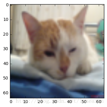
# Plot learning curve (with costs)
costs = np.squeeze(d['costs'])
plt.plot(costs)
plt.ylabel('cost')
plt.xlabel('iterations (per hundreds)')
plt.title("Learning rate =" + str(d["learning_rate"]))
plt.show()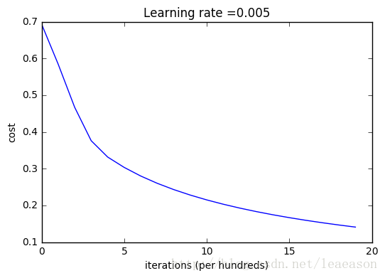
6 - Further analysis (optional/ungraded exercise)
examine possible choices for the learning rate αlearning_rates = [0.01, 0.001, 0.005,0.0001]
models = {}
for i in learning_rates:
print ("learning rate is: " + str(i))
models[str(i)] = model(train_set_x, train_set_y, test_set_x, test_set_y, num_iterations = 1500, learning_rate = i, print_cost = False)
print ('\n' + "-------------------------------------------------------" + '\n')
for i in learning_rates:
plt.plot(np.squeeze(models[str(i)]["costs"]), label= str(models[str(i)]["learning_rate"]))
plt.ylabel('cost')
plt.xlabel('iterations')
legend = plt.legend(loc='upper center', shadow=True)
frame = legend.get_frame()
frame.set_facecolor('0.90')
plt.show()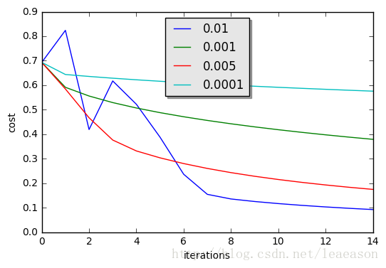
7 - Test with your own image (optional/ungraded exercise)
## START CODE HERE ## (PUT YOUR IMAGE NAME)
my_image = "cat.2.jpg"   # change this to the name of your image file
## END CODE HERE ##
# We preprocess the image to fit your algorithm.
fname = "images/" + my_image
image = np.array(ndimage.imread(fname, flatten=False))
my_image = scipy.misc.imresize(image, size=(num_px,num_px)).reshape((1, num_px*num_px*3)).T
my_predicted_image = predict(d["w"], d["b"], my_image
plt.imshow(image)
print("y = " + str(np.squeeze(my_predicted_image)) + ", your algorithm predicts a \"" + classes[int(np.squeeze(my_predicted_image)),].decode("utf-8") +  "\" picture.")

相关文章推荐
- [置顶] Coursera-Deep Learning Specialization 课程之(四):Convolutional Neural Networks: -weak2编程作业
- Coursera-Deep Learning Specialization 课程之(一):Neural Networks and Deep Learning-weak1
- [置顶] Coursera-Deep Learning Specialization 课程之(一):Neural Networks and Deep Learning-weak3编程作业
- Coursera-Deep Learning Specialization 课程之(一):Neural Networks and Deep Learning-weak2
- Coursera-Deep Learning Specialization 课程之(一):Neural Networks and Deep Learning-weak4编程作业
- [置顶] Coursera-Deep Learning Specialization 课程之(四):Convolutional Neural Networks: -weak1编程作业
- [置顶] Coursera-Deep Learning Specialization 课程之(四):Convolutional Neural Networks: -weak3编程作业
- Coursera-Deep Learning Specialization 课程之(二):Improving Deep Neural Networks: -weak2编程作业
- 【吴恩达 Coursera深度学习课程】 Neural Networks and Deep Learning 第一周课后习题
- [置顶] Coursera-Deep Learning Specialization 课程之(四):Convolutional Neural Networks: -weak4编程作业
- neural networks and deep learning 吴恩达coursera公开课
- Coursera上DeepLearning系列课程第一课Neural Network and Deep Learning课程PPT和笔记
- Coursera-Deep Learning Specialization 课程之(二):Improving Deep Neural Networks: -weak1编程作业
- [置顶] Coursera-Deep Learning Specialization 课程之(五):Sequence Models: -weak1编程作业
- Coursera-Deep Learning Specialization 课程之(二):Improving Deep Neural Networks: -weak3编程作业
- [置顶] Coursera-Deep Learning Specialization 课程之(五):Sequence Models: -weak1编程作业 (第二部分)
- [置顶] Coursera-Deep Learning Specialization 课程之(五):Sequence Models: -weak1编程作业 (第三部分)
- 读书笔记--Neural Networks and Deep Learning(CH1)
- Neural Networks and Deep Learning-读书笔记
- 【deeplearning.ai】Neural Networks and Deep Learning——浅层神经网络