员工离职预测
2017-10-16 14:35
387 查看
员工离职预测
library(dplyr)library(psych)library(ggplot2)library(randomForest)str(train)'data.frame': 1100 obs. of 31 variables: $ X...Age : int 37 54 34 39 28 24 29 36 33 34 ... $ Attrition : int 0 0 1 0 1 0 0 0 0 0 ... $ BusinessTravel : Factor w/ 3 levels "Non-Travel","Travel_Frequently",..: 3 2 2 3 2 3 3 3 3 3 ... $ Department : Factor w/ 3 levels "Human Resources",..: 2 2 2 2 2 3 2 3 2 2 ... $ DistanceFromHome : int 1 1 7 1 1 4 9 2 4 2 ... $ Education : int 4 4 3 1 3 1 5 2 4 4 ... $ EducationField : Factor w/ 6 levels "Human Resources",..: 2 2 2 2 4 4 5 4 4 6 ... $ EmployeeNumber : int 77 1245 147 1026 1111 1445 455 513 305 1383 ... $ EnvironmentSatisfaction : int 1 4 1 4 1 4 2 2 3 3 ... $ Gender : Factor w/ 2 levels "Female","Male": 2 1 2 1 2 1 2 2 1 1 ... $ JobInvolvement : int 2 3 1 2 2 3 2 2 2 3 ... $ JobLevel : int 2 3 2 4 1 2 1 3 1 2 ... $ JobRole : Factor w/ 9 levels "Healthcare Representative",..: 5 5 3 5 3 8 3 8 7 1 ... $ JobSatisfaction : int 3 3 3 4 2 3 4 3 2 4 ... $ MaritalStatus : Factor w/ 3 levels "Divorced","Married",..: 1 1 3 2 1 2 3 2 2 3 ... $ MonthlyIncome : int 5993 10502 6074 12742 2596 4162 3983 7596 2622 6687 ... $ NumCompaniesWorked : int 1 7 1 1 1 1 0 1 6 1 ... $ Over18 : Factor w/ 1 level "Y": 1 1 1 1 1 1 1 1 1 1 ... $ OverTime : Factor w/ 2 levels "No","Yes": 1 1 2 1 1 2 1 1 1 1 ... $ PercentSalaryHike : int 18 17 24 16 15 12 17 13 21 11 ... $ PerformanceRating : int 3 3 4 3 3 3 3 3 4 3 ... $ RelationshipSatisfaction: int 3 1 4 3 1 3 3 2 4 4 ... $ StandardHours : int 80 80 80 80 80 80 80 80 80 80 ... $ StockOptionLevel : int 1 1 0 1 2 2 0 2 0 0 ... $ TotalWorkingYears : int 7 33 9 21 1 5 4 10 7 14 ... $ TrainingTimesLastYear : int 2 2 3 3 2 3 2 2 3 2 ... $ WorkLifeBalance : int 4 1 3 3 3 3 3 3 3 4 ... $ YearsAtCompany : int 7 5 9 21 1 5 3 10 3 14 ... $ YearsInCurrentRole : int 5 4 7 6 0 4 2 9 2 11 ... $ YearsSinceLastPromotion : int 0 1 0 11 0 0 2 9 1 4 ... $ YearsWithCurrManager : int 7 4 6 8 0 3 2 0 1 11 ...
describe(train)
vars    n    mean      sd median trimmed     mad  min   max range  skew kurtosis     se
X...Age                     1 1100   37.00    9.04   36.0   36.51    8.90   18    60    42  0.44    -0.43   0.27
Attrition                   2 1100    0.16    0.37    0.0    0.08    0.00    0     1     1  1.83     1.36   0.01
BusinessTravel*             3 1100    2.62    0.66    3.0    2.77    0.00    1     3     2 -1.47     0.81   0.02
Department*                 4 1100    2.26    0.52    2.0    2.25    0.00    1     3     2  0.23    -0.41   0.02
DistanceFromHome            5 1100    9.43    8.20    7.0    8.36    7.41    1    29    28  0.91    -0.35   0.25
Education                   6 1100    2.92    1.02    3.0    2.99    1.48    1     5     4 -0.30    -0.55   0.03
EducationField*             7 1100    3.22    1.32    3.0    3.06    1.48    1     6     5  0.58    -0.65   0.04
EmployeeNumber              8 1100 1028.16  598.92 1026.5 1027.04  782.81    1  2065  2064  0.02    -1.22  18.06
EnvironmentSatisfaction     9 1100    2.73    1.10    3.0    2.78    1.48    1     4     3 -0.33    -1.21   0.03
Gender*                    10 1100    1.59    0.49    2.0    1.62    0.00    1     2     1 -0.38    -1.86   0.01
JobInvolvement             11 1100    2.73    0.71    3.0    2.74    0.00    1     4     3 -0.54     0.34   0.02
JobLevel                   12 1100    2.05    1.11    2.0    1.89    1.48    1     5     4  1.04     0.40   0.03
JobRole*                   13 1100    5.43    2.46    6.0    5.59    2.97    1     9     8 -0.34    -1.22   0.07
JobSatisfaction            14 1100    2.73    1.11    3.0    2.79    1.48    1     4     3 -0.33    -1.24   0.03
MaritalStatus*             15 1100    2.11    0.73    2.0    2.14    1.48    1     3     2 -0.18    -1.12   0.02
MonthlyIncome              16 1100 6483.62 4715.29 4857.0 5639.41 3166.09 1009 19999 18990  1.38     1.04 142.17
NumCompaniesWorked         17 1100    2.68    2.51    2.0    2.35    1.48    0     9     9  1.03    -0.02   0.08
Over18*                    18 1100    1.00    0.00    1.0    1.00    0.00    1     1     0   NaN      NaN   0.00
OverTime*                  19 1100    1.28    0.45    1.0    1.22    0.00    1     2     1  0.99    -1.02   0.01
PercentSalaryHike          20 1100   15.24    3.63   14.0   14.85    2.97   11    25    14  0.79    -0.35   0.11
PerformanceRating          21 1100    3.15    0.36    3.0    3.07    0.00    3     4     1  1.93     1.72   0.01
RelationshipSatisfaction   22 1100    2.70    1.10    3.0    2.75    1.48    1     4     3 -0.29    -1.23   0.03
StandardHours              23 1100   80.00    0.00   80.0   80.00    0.00   80    80     0   NaN      NaN   0.00
StockOptionLevel           24 1100    0.79    0.84    1.0    0.67    1.48    0     3     3  0.95     0.34   0.03
TotalWorkingYears          25 1100   11.22    7.83   10.0   10.27    5.93    0    40    40  1.15     0.99   0.24
TrainingTimesLastYear      26 1100    2.81    1.29    3.0    2.74    1.48    0     6     6  0.50     0.49   0.04
WorkLifeBalance            27 1100    2.75    0.70    3.0    2.76    0.00    1     4     3 -0.60     0.47   0.02
YearsAtCompany             28 1100    7.01    6.22    5.0    5.94    4.45    0    37    37  1.81     4.01   0.19
YearsInCurrentRole         29 1100    4.21    3.62    3.0    3.83    4.45    0    18    18  0.95     0.61   0.11
YearsSinceLastPromotion    30 1100    2.23    3.31    1.0    1.49    1.48    0    15    15  1.94     3.30   0.10
YearsWithCurrManager       31 1100    4.12    3.60    3.0    3.76    4.45    0    17    17  0.86     0.26   0.11
#删除 常量
name<-names(train)
train<-train[name!="Over18" & name!="StandardHours" & name!="EmployeeNumber"]
#重编码
train$Gender<-as.integer(train$Gender)-1
train$OverTime<-as.integer(train$OverTime)-1
#Age 和 Attrition
ggplot(train, aes(X...Age, fill = factor(Attrition))) +
geom_histogram(bins=30) +
facet_grid(.~Gender)+
labs(fill="Attrition")+ xlab("Age")+ylab("Total Count")
#小结:
#小结:train$X...Age[train$X...Age>=18 & train$X...Age <25]<-1 train$X...Age[train$X...Age>=25 & train$X...Age <35]<-2 train$X...Age[train$X...Age>=35 & train$X...Age <45]<-3 train$X...Age[train$X...Age>=45 & train$X...Age <55]<-4 train$X...Age[train$X...Age>=55 ]<-5#Department 和 JobLevel
ggplot(train, aes(x = JobLevel, fill = as.factor(Attrition))) +
 geom_bar() +
 facet_wrap(~ Department)+

xlab("Job Level")+

ylab("Total Count")+

labs(fill = "Attrition")
train$Department<-as.character(train$Department)
train$Department[train$Department=="Human Resources"]<-"1"
train$Department[train$Department=="Sales"]<-"2"
train$Department[train$Department=="Research & Development"]<-"3"
train$Department<-as.integer(train$Department)
#小结:不同部门相同级别之间存在明显差异,研发部门1,2级别和销售部1,2,3级别流动性较大。#Department 和 BusinessTravel
ggplot(train, aes(x = BusinessTravel, fill = as.factor(Attrition))) +
geom_bar() +
facet_wrap(~ Department)+
xlab("BusinessTravel")+
ylab("Total Count")+
labs(fill = "Attrition")
train$BusinessTravel<-as.character(train$BusinessTravel)
train$BusinessTravel[train$BusinessTravel=="Non-Travel"]<-"1"
train$BusinessTravel[train$BusinessTravel=="Travel_Frequently"]<-"2"
train$BusinessTravel[train$BusinessTravel=="Travel_Rarely"]<-"3"
train$BusinessTravel<-as.integer(train$BusinessTravel)
#小结:是否经常出差,并不是影响离职的关键因素,但偶然出差的员工离职率最高。研发部、销售部、人力资源部依次下降。#EducationField 和 Attrition
ggplot(train,aes(EducationField,fill=as.factor(Attrition)))+
geom_bar(stat="count",position="dodge")+
xlab("EducationField")+
ylab("Total Count")+
labs(fill="Attrition")
#小结:专业领域和离职之间无明显关系#MaritalStatus 和 Attrition
ggplot(train,aes(MaritalStatus,fill=as.factor(Attrition)))+
geom_bar(stat="count",position="dodge")+
xlab("MaritalStatus")+
ylab("Total Count")+
labs(fill="Attrition")
train$MaritalStatus<-as.character(train$MaritalStatus)
train$MaritalStatus[train$MaritalStatus=="Divorced"]<-1
train$MaritalStatus[train$MaritalStatus=="Married"]<-2
train$MaritalStatus[train$MaritalStatus=="Single"]<-3
train$MaritalStatus<-as.integer(train$MaritalStatus)
#小结:婚姻情况和离职有一点关系#EnvironmentSatisfaction 和 Attrition
ggplot(train, aes(x = EnvironmentSatisfaction, fill = as.factor(Attrition))) +
geom_bar() +
facet_wrap(~ JobLevel)+
xlab("JobLevel")+
ylab("Total Count")+
labs(fill = "Attrition")
#小结:满意度和离职之间无明显关系#MonthlyIncome 和 Attrition
ggplot(train,aes(MonthlyIncome, fill = factor(Attrition))) +
geom_density(alpha = 0.8)+
labs(fill="Attrition")
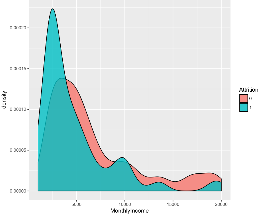 #小结:低收入者明显在职意向不稳定
train$MonthlyIncome[train$MonthlyIncome<=3000]<-1
train$MonthlyIncome[train$MonthlyIncome>3000 & train$MonthlyIncome<=6000]<-2
train$MonthlyIncome[train$MonthlyIncome>6000 & train$MonthlyIncome<=9000]<-3
train$MonthlyIncome[train$MonthlyIncome>9000 & train$MonthlyIncome<=12000]<-4
train$MonthlyIncome[train$MonthlyIncome>12000 & train$MonthlyIncome<=17000]<-5
train$MonthlyIncome[train$MonthlyIncome>17000]<-6
#关联关系
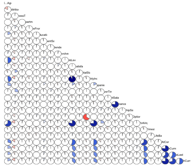
corrgram(train[,-c(7,12)],lower.panel=panel.pie,upper.panel=NULL)
 #抽样
#抽样set.seed(1)ind<-sample(2,nrow(train),replace=TRUE,prob=c(0.7,0.3))train.df<-train[ind==1,]test.df<-train[ind==2,]
#随机森林
rf<-randomForest(factor(Attrition)~.,data=train.df)varImpPlot(rf)
 #准确率
#准确率prediction <- predict(rf,newdata=test.df,type="response")misClasificError <- mean(prediction != test.df$Attrition)print(paste('Accuracy',1-misClasificError))[1] "Accuracy 0.876506024096386"#逻辑回归gf<-glm(Attrition~.,data=train.df,family = binomial(link=logit))summary(gf)Call:glm(formula = Attrition ~ ., family = binomial(link = logit),data = train.df)Deviance Residuals:Min 1Q Median 3Q Max-1.6113 -0.5048 -0.2459 -0.0860 3.4737Coefficients:Estimate Std. Error z value Pr(>|z|)(Intercept) -1.31753 3.58064 -0.368 0.712903X...Age -0.36136 0.17640 -2.049 0.040508 *BusinessTravel 0.05908 0.20110 0.294 0.768928Department 0.39070 0.93431 0.418 0.675820DistanceFromHome 0.05274 0.01486 3.550 0.000386 ***Education -0.17039 0.12279 -1.388 0.165239EducationFieldLife Sciences -0.43924 1.20639 -0.364 0.715785EducationFieldMarketing 0.14995 1.25574 0.119 0.904948EducationFieldMedical -0.55928 1.20602 -0.464 0.642835EducationFieldOther 0.07420 1.32247 0.056 0.955256EducationFieldTechnical Degree 0.62904 1.22665 0.513 0.608084EnvironmentSatisfaction -0.50299 0.11646 -4.319 1.57e-05 ***Gender 0.49495 0.26618 1.859 0.062965 .JobInvolvement -0.67266 0.17777 -3.784 0.000154 ***JobLevel -0.18383 0.39279 -0.468 0.639777JobRoleHuman Resources 2.92472 2.10883 1.387 0.165474JobRoleLaboratory Technician 2.11121 0.82806 2.550 0.010785 *JobRoleManager 2.09557 1.12796 1.858 0.063193 .JobRoleManufacturing Director 1.22695 0.84649 1.449 0.147211JobRoleResearch Director 1.49258 1.17894 1.266 0.205501JobRoleResearch Scientist 1.44543 0.82801 1.746 0.080868 .JobRoleSales Executive 2.17131 1.20040 1.809 0.070479 .JobRoleSales Representative 3.29933 1.28712 2.563 0.010367 *JobSatisfaction -0.63089 0.11767 -5.361 8.26e-08 ***MaritalStatus 0.94530 0.25146 3.759 0.000170 ***MonthlyIncome -0.03459 0.24924 -0.139 0.889628NumCompaniesWorked 0.13934 0.05418 2.572 0.010119 *OverTime 2.18546 0.27520 7.941 2.00e-15 ***PercentSalaryHike -0.05939 0.05572 -1.066 0.286492PerformanceRating 0.86885 0.55923 1.554 0.120266RelationshipSatisfaction -0.33278 0.11625 -2.863 0.004201 **StockOptionLevel 0.01585 0.21361 0.074 0.940835TotalWorkingYears -0.04047 0.04220 -0.959 0.337593TrainingTimesLastYear -0.15291 0.10058 -1.520 0.128425WorkLifeBalance -0.21648 0.16944 -1.278 0.201398YearsAtCompany 0.07885 0.05340 1.477 0.139745YearsInCurrentRole -0.13861 0.06449 -2.149 0.031612 *YearsSinceLastPromotion 0.14022 0.05867 2.390 0.016857 *YearsWithCurrManager -0.11790 0.06483 -1.819 0.068956 .---Signif. codes: 0 '***' 0.001 '**' 0.01 '*' 0.05 '.' 0.1 ' ' 1(Dispersion parameter for binomial family taken to be 1)Null deviance: 717.22 on 767 degrees of freedomResidual deviance: 457.00 on 729 degrees of freedomAIC: 535Number of Fisher Scoring iterations: 6#准确率
prediction <- predict(gf,newdata=test.df,type="response")prediction <- ifelse(prediction > 0.5,1,0)misClasificError <- mean(prediction != test.df$Attrition)print(paste('Accuracy',1-misClasificError))[1] "Accuracy 0.858433734939759"

相关文章推荐
- R:员工离职预测实战
- 《用python进行员工离职原因分析与预测-----小象学院公开课》
- 转:kaggle案例:员工离职预测 (附视频)
- R语言-向量机-员工离职预测训练赛
- 无征兆离职——你属于不会哭的孩子类型员工吗?
- 从现代人力资源管理角度看员工离职
- 马云说,离职的员工林林总总
- 马云说:员工的离职原因林林总总,只有两点最真实
- 百度员工离职总结:如何做个好员工
- 百度员工离职总结:如何做个好员工?
- 百度员工离职总结:如何做个好员工
- 百度员工离职总结:如何做个好员工
- 百度员工离职总结:如何做个好员工?
- 一个7年老员工的离职总结:如何打造一个最强大的“自我”
- BD资深员工离职总结:资质平庸的人如何做一个好员工?
- 你造吗?70%的优秀员工是这样离职的
- 前亚马逊员工离职创业 10家创业公司各具特色
- 从员工离职后有想来的感想
- 公司的秘密:如何让员工主动离职?HR常用这8招