（二）非线性循环神经网络（RNN）

这篇教程是翻译Peter Roelants写的循环神经网络教程，作者已经授权翻译，这是原文。

该教程将介绍如何实现一个循环神经网络（RNN），一共包含两部分。你可以在以下链接找到完整内容。

（一）线性循环神经网络（RNN）

（二）非线性循环神经网络（RNN）

非线性循环神经网络应用于二进制相加

本教程主要包含两部分：

利用张量存储数据

利用弹性反向传播和动量方法进行优化

在第一部分中，我们已经学习了一个简单的线性循环神经网络。在这一部分中，我们将利用非线性函数来设计一个非线性的循环神经网络，并且实现一个二进制相加的功能。

我们先导入教程需要的软件包：

import itertools
import numpy as np
import matplotlib
import matplotlib.pyplot as plt

定义数据集

在这个教程中，我们训练的数据集是2000个数据，在程序中用

create_dataset

函数产生。每个训练样本都是有两部分

(Xi1, Xi2)

组成，每一部分是一个7位的二进制表示，分别由6位的二进制和最右边一位的0组成（最右边的0是为了防止二进制相加溢出）。预测目标

ti

也是一个7位的二进制表示，即

ti = Xi1 + Xi2

。我们之所以从左到右编码二进制，是因为我们的RNN网络是从左到右进行计算的。

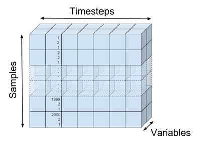
输入数据和预测结果都是被存储在三维张量里，比如下图表示了我们的训练数据

(X_train, T_train)

的维度表示。第一维度表示一共有多少组数据（我们第一维度的值是 2000），第二维度表示的是每个时间步长上面的取值，一共7个时间步长，第三维度表示RNN输入单元神经元的个数（该教程设置的是2个神经元）。下图就是输入张量

X_train

的可视化展示：



输入张量可视化表示

下面代码定义了输入数据集：

# Create dataset
nb_train = 2000  # Number of training samples
# Addition of 2 n-bit numbers can result in a n+1 bit number
sequence_len = 7  # Length of the binary sequence

def create_dataset(nb_samples, sequence_len):
"""Create a dataset for binary addition and return as input, targets."""
max_int = 2**(sequence_len-1) # Maximum integer that can be added
format_str = '{:0' + str(sequence_len) + 'b}' # Transform integer in binary format
nb_inputs = 2  # Add 2 binary numbers
nb_outputs = 1  # Result is 1 binary number
X = np.zeros((nb_samples, sequence_len, nb_inputs))  # Input samples
T = np.zeros((nb_samples, sequence_len, nb_outputs))  # Target samples
# Fill up the input and target matrix
for i in xrange(nb_samples):
# Generate random numbers to add
nb1 = np.random.randint(0, max_int)
nb2 = np.random.randint(0, max_int)
# Fill current input and target row.
# Note that binary numbers are added from right to left, but our RNN reads
#  from left to right, so reverse the sequence.
X[i,:,0] = list(reversed([int(b) for b in format_str.format(nb1)]))
X[i,:,1] = list(reversed([int(b) for b in format_str.format(nb2)]))
T[i,:,0] = list(reversed([int(b) for b in format_str.format(nb1+nb2)]))
return X, T

# Create training samples
X_train, T_train = create_dataset(nb_train, sequence_len)
print('X_train shape: {0}'.format(X_train.shape))
print('T_train shape: {0}'.format(T_train.shape))

X_train shape: (2000, 7, 2)
T_train shape: (2000, 7, 1)

二进制相加

如果需要理解循环神经网络从输入数据流到输出数据流的一整个形式，那么二进制相加将是一个很好的例子。循环神经网络需要学习两件事：第一，怎么去将上一次的运算状态传递到下一次的运算中去；第二，根据输入数据和上一步的输入状态值（也就是记忆），去判断什么时候应该输出0，什么时候应该输出1。

下面代码将二进制相加结果做了一个可视化：

# Show an example input and target
def printSample(x1, x2, t, y=None):
"""Print a sample in a more visual way."""
x1 = ''.join([str(int(d)) for d in x1])
x2 = ''.join([str(int(d)) for d in x2])
t = ''.join([str(int(d[0])) for d in t])
if not y is None:
y = ''.join([str(int(d[0])) for d in y])
print('x1:   {:s}   {:2d}'.format(x1, int(''.join(reversed(x1)), 2)))
print('x2: + {:s}   {:2d} '.format(x2, int(''.join(reversed(x2)), 2)))
print('      -------   --')
print('t:  = {:s}   {:2d}'.format(t, int(''.join(reversed(t)), 2)))
if not y is None:
print('y:  = {:s}'.format(t))

# Print the first sample
printSample(X_train[0,:,0], X_train[0,:,1], T_train[0,:,:])

x1: 1010010 37
x2: + 1101010 43
--------------------
t: = 0000101 80

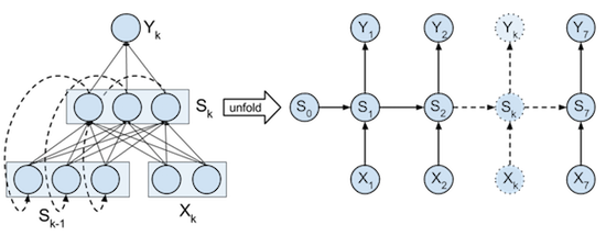
循环神经网络架构

在这个教程中，对于每个时间点，我们设计的循环神经网络有2个输入神经元，之后将它们转换成状态值，最后输出一个单独的预测概率值。当前的时间点是1（而不是0）。由输入数据转换成的状态值，它的作用是记住一部分信息，以便于网络与预测下一步应该输出什么。

网上有很多的方法，可以将我们设计的RNN进行可视化展示，我们还是利用在第一部分中的展示方法，将我们的RNN架构进行战术，如下图：



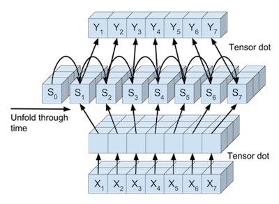
或者，我们还能将完整的输入数据，完整的状态值和完整的预测结果进行可视化，输入数据张量可以被并行映射到状态值张量，状态值张量也可以被并行映射到每一个时间点的预测值张量。如下图：



在代码中，每一个映射过程被抽象成了一个类。在每一个类中，都有一个

forward

函数用来计算BP算法中的前向传播，

backward

函数来计算BP算法中的反向传播。

RNN的计算过程

线性转换
在神经网络中，将输入数据映射到下一层的常用方法是矩阵相乘并且加上偏差项，最后利用一个非线性函数进行激活操作。在这篇教程中，二维的输入数据

(Xik1, Xik2)

，通过一个

2*3

的链接矩阵和长度是3的偏差向量映射到状态层，即下一层。在状态反馈之前，三维的状态值，将会通过一个

3*1

的链接矩阵和长度是1的偏差向量映射到输出层，即得到输出概率。

因为我们想在一个计算步骤中，将训练样本中的每个样本在每个时间点都进行状态映射，所以我们将使用 Numpy 中的

tensordot

函数，去实现这个相乘的操作。这个函数需要输入2个张量和指定需要累加的轴。比如，输入数据为

shape(X) = (2000, 7, 2)

，状态值为

shape(S) = (2000, 7, 3)

，链接矩阵为

shape(W) = (2, 3)

，那么我们可以得到公式

S = tensordot(X, W, axes = ((-1), (0))

。这个公式会把

X

的最后一维

(-1)

和

W

的第零维度进行相乘累加，最后得到一个维度是

(2000, 7, 3)

的张量。

这个线性转换可以用在输入数据

X

到状态层

S

的映射，也可以用在状态层

S

到输出层

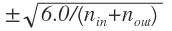
Y

的映射。在代码的

TensorLinear

类中，实现了这个线性转换，还实现了它的梯度。根据Xavier Glorot的建议，权重初始值是一个均匀分布，数据范围是：



Logitstic分类
Logistic分类函数将被在输出层使用，用来得到输出的概率值，在

LogisticClassifier

函数中实现了它的损失函数和梯度。

# Define the linear tensor transformation layer
class TensorLinear(object):
"""The linear tensor layer applies a linear tensor dot product and a bias to its input."""
def __init__(self, n_in, n_out, tensor_order, W=None, b=None):
"""Initialse the weight W and bias b parameters."""
a = np.sqrt(6.0 / (n_in + n_out))
self.W = (np.random.uniform(-a, a, (n_in, n_out)) if W is None else W)
self.b = (np.zeros((n_out)) if b is None else b)  # Bias paramters
self.bpAxes = tuple(range(tensor_order-1))  # Axes summed over in backprop

def forward(self, X):
"""Perform forward step transformation with the help of a tensor product."""
# Same as: Y[i,j,:] = np.dot(X[i,j,:], self.W) + self.b (for i,j in X.shape[0:1])
# Same as: Y = np.einsum('ijk,kl->ijl', X, self.W) + self.b
return np.tensordot(X, self.W, axes=((-1),(0))) + self.b

def backward(self, X, gY):
"""Return the gradient of the parmeters and the inputs of this layer."""
# Same as: gW = np.einsum('ijk,ijl->kl', X, gY)
# Same as: gW += np.dot(X[:,j,:].T, gY[:,j,:]) (for i,j in X.shape[0:1])
gW = np.tensordot(X, gY, axes=(self.bpAxes, self.bpAxes))
gB = np.sum(gY, axis=self.bpAxes)
# Same as: gX = np.einsum('ijk,kl->ijl', gY, self.W.T)
# Same as: gX[i,j,:] = np.dot(gY[i,j,:], self.W.T) (for i,j in gY.shape[0:1])
gX = np.tensordot(gY, self.W.T, axes=((-1),(0)))
return gX, gW, gB

# Define the logistic classifier layer
class LogisticClassifier(object):
"""The logistic layer applies the logistic function to its inputs."""

def forward(self, X):
"""Perform the forward step transformation."""
return 1 / (1 + np.exp(-X))

def backward(self, Y, T):
"""Return the gradient with respect to the cost function at the inputs of this layer."""
# Normalise of the number of samples and sequence length.
return (Y - T) / (Y.shape[0] * Y.shape[1])

def cost(self, Y, T):
"""Compute the cost at the output."""
# Normalise of the number of samples and sequence length.
# Add a small number (1e-99) because Y can become 0 if the network learns
#  to perfectly predict the output. log(0) is undefined.
return - np.sum(np.multiply(T, np.log(Y+1e-99)) + np.multiply((1-T), np.log(1-Y+1e-99))) / (Y.shape[0] * Y.shape[1])

展开循环神经网络的中间状态
在上一部分教程中，我们知道随着时间步长，我们需要把循环状态进行展开处理。在代码中，

RecurrentStateUnfold

类实现了这个展开的BPTT算法。这个类包含了前一状态层到当前状态层的权重，偏差单元，当然也实现了权重初始化和优化函数。

在

RecurrentStateUnfold

类中，

forward

函数实现了随着时间步长，状态函数的迭代更新。

backward

函数实现了每个输出状态值的梯度。在每个时间点

k

上，输出层

Y

的梯度还需要加上上一状态的梯度之和。权重项和偏差项的梯度需要将所有时间点上面的权重项和偏差项的梯度都进行累加，因为在每一个时间点它们的值都是共享的。在时间点

k = 0

，最后状态的梯度需要去优化初始的状态

S0

，因为初始状体的梯度是

∂ξ/∂S0

。

RecurrentStateUnfold

类需要使用

RecurrentStateUpdate

类。这个类中的

forward

方法实现了将

k-1

的状态和 input 输入进行联合计算得到

k

时刻的状态值。

backward

方法实现了BPTT算法。在

RecurrentStateUpdate

类中实现的非线性激活函数是hyperbolic tangent (tanh)函数，这个函数的取值范围是从 -1 到 +1。这个函数在

TanH

类中实现了。

# Define tanh layer
class TanH(object):
"""TanH applies the tanh function to its inputs."""

def forward(self, X):
"""Perform the forward step transformation."""
return np.tanh(X)

def backward(self, Y, output_grad):
"""Return the gradient at the inputs of this layer."""
gTanh = 1.0 - np.power(Y,2)
return np.multiply(gTanh, output_grad)

# Define internal state update layer
class RecurrentStateUpdate(object):
"""Update a given state."""
def __init__(self, nbStates, W, b):
"""Initialse the linear transformation and tanh transfer function."""
self.linear = TensorLinear(nbStates, nbStates, 2, W, b)
self.tanh = TanH()

def forward(self, Xk, Sk):
"""Return state k+1 from input and state k."""
return self.tanh.forward(Xk + self.linear.forward(Sk))

def backward(self, Sk0, Sk1, output_grad):
"""Return the gradient of the parmeters and the inputs of this layer."""
gZ = self.tanh.backward(Sk1, output_grad)
gSk0, gW, gB = self.linear.backward(Sk0, gZ)
return gZ, gSk0, gW, gB

# Define layer that unfolds the states over time
class RecurrentStateUnfold(object):
"""Unfold the recurrent states."""
def __init__(self, nbStates, nbTimesteps):
" Initialse the shared parameters, the inital state and state update function."
a = np.sqrt(6.0 / (nbStates * 2))
self.W = np.random.uniform(-a, a, (nbStates, nbStates))
self.b = np.zeros((self.W.shape[0]))  # Shared bias
self.S0 = np.zeros(nbStates)  # Initial state
self.nbTimesteps = nbTimesteps  # Timesteps to unfold
self.stateUpdate = RecurrentStateUpdate(nbStates, self.W, self.b)  # State update function

def forward(self, X):
"""Iteratively apply forward step to all states."""
S = np.zeros((X.shape[0], X.shape[1]+1, self.W.shape[0]))  # State tensor
S[:,0,:] = self.S0  # Set initial state
for k in range(self.nbTimesteps):
# Update the states iteratively
S[:,k+1,:] = self.stateUpdate.forward(X[:,k,:], S[:,k,:])
return S

def backward(self, X, S, gY):
"""Return the gradient of the parmeters and the inputs of this layer."""
gSk = np.zeros_like(gY[:,self.nbTimesteps-1,:])  # Initialise gradient of state outputs
gZ = np.zeros_like(X)  # Initialse gradient tensor for state inputs
gWSum = np.zeros_like(self.W)  # Initialise weight gradients
gBSum = np.zeros_like(self.b)  # Initialse bias gradients
# Propagate the gradients iteratively
for k in range(self.nbTimesteps-1, -1, -1):
# Gradient at state output is gradient from previous state plus gradient from output
gSk += gY[:,k,:]
# Propgate the gradient back through one state
gZ[:,k,:], gSk, gW, gB = self.stateUpdate.backward(S[:,k,:], S[:,k+1,:], gSk)
gWSum += gW  # Update total weight gradient
gBSum += gB  # Update total bias gradient
gS0 = np.sum(gSk, axis=0)  # Get gradient of initial state over all samples
return gZ, gWSum, gBSum, gS0

整个网络
在

RnnBinaryAdder

类中，实现了整个二进制相加的网络过程。它在创建的时候，同时初始化了所有的网络参数。

forward

方法实现了整个网络的前向传播过程，

backward

方法实现了整个网络的梯度更新和反向传播过程。

getParamGrads

方法计算了每一个参数的梯度，并且作为一个列表进行返回。

get_params_iter

方法是将参数做一个索引排序，使得参数的梯度按照一定的顺序返回。

# Define the full network
class RnnBinaryAdder(object):
"""RNN to perform binary addition of 2 numbers."""
def __init__(self, nb_of_inputs, nb_of_outputs, nb_of_states, sequence_len):
"""Initialse the network layers."""
self.tensorInput = TensorLinear(nb_of_inputs, nb_of_states, 3)  # Input layer
self.rnnUnfold = RecurrentStateUnfold(nb_of_states, sequence_len)  # Recurrent layer
self.tensorOutput = TensorLinear(nb_of_states, nb_of_outputs, 3)  # Linear output transform
self.classifier = LogisticClassifier()  # Classification output

def forward(self, X):
"""Perform the forward propagation of input X through all layers."""
recIn = self.tensorInput.forward(X)  # Linear input transformation
# Forward propagate through time and return states
S = self.rnnUnfold.forward(recIn)
Z = self.tensorOutput.forward(S[:,1:sequence_len+1,:])  # Linear output transformation
Y = self.classifier.forward(Z)  # Get classification probabilities
# Return: input to recurrent layer, states, input to classifier, output
return recIn, S, Z, Y

def backward(self, X, Y, recIn, S, T):
"""Perform the backward propagation through all layers.
Input: input samples, network output, intput to recurrent layer, states, targets."""
gZ = self.classifier.backward(Y, T)  # Get output gradient
gRecOut, gWout, gBout = self.tensorOutput.backward(S[:,1:sequence_len+1,:], gZ)
# Propagate gradient backwards through time
gRnnIn, gWrec, gBrec, gS0 = self.rnnUnfold.backward(recIn, S, gRecOut)
gX, gWin, gBin = self.tensorInput.backward(X, gRnnIn)
# Return the parameter gradients of: linear output weights, linear output bias,
#  recursive weights, recursive bias, linear input weights, linear input bias, initial state.
return gWout, gBout, gWrec, gBrec, gWin, gBin, gS0

def getOutput(self, X):
"""Get the output probabilities of input X."""
recIn, S, Z, Y = self.forward(X)
return Y  # Only return the output.

def getBinaryOutput(self, X):
"""Get the binary output of input X."""
return np.around(self.getOutput(X))

def getParamGrads(self, X, T):
"""Return the gradients with respect to input X and target T as a list.
The list has the same order as the get_params_iter iterator."""
recIn, S, Z, Y = self.forward(X)
gWout, gBout, gWrec, gBrec, gWin, gBin, gS0 = self.backward(X, Y, recIn, S, T)
return [g for g in itertools.chain(
np.nditer(gS0),
np.nditer(gWin),
np.nditer(gBin),
np.nditer(gWrec),
np.nditer(gBrec),
np.nditer(gWout),
np.nditer(gBout))]

def cost(self, Y, T):
"""Return the cost of input X w.r.t. targets T."""
return self.classifier.cost(Y, T)

def get_params_iter(self):
"""Return an iterator over the parameters.
The iterator has the same order as get_params_grad.
The elements returned by the iterator are editable in-place."""
return itertools.chain(
np.nditer(self.rnnUnfold.S0, op_flags=['readwrite']),
np.nditer(self.tensorInput.W, op_flags=['readwrite']),
np.nditer(self.tensorInput.b, op_flags=['readwrite']),
np.nditer(self.rnnUnfold.W, op_flags=['readwrite']),
np.nditer(self.rnnUnfold.b, op_flags=['readwrite']),
np.nditer(self.tensorOutput.W, op_flags=['readwrite']),
np.nditer(self.tensorOutput.b, op_flags=['readwrite']))

梯度检查

我们需要将网络求得的梯度和进行数值计算得到的梯度进行比较，从而判断梯度是否计算正确，我们在这篇博客中已经详细介绍了如何进行梯度检查，如果还有不明白，可以查看这篇博客。

# Do gradient checking
# Define an RNN to test
RNN = RnnBinaryAdder(2, 1, 3, sequence_len)
# Get the gradients of the parameters from a subset of the data
backprop_grads = RNN.getParamGrads(X_train[0:100,:,:], T_train[0:100,:,:])

eps = 1e-7  # Set the small change to compute the numerical gradient
# Compute the numerical gradients of the parameters in all layers.
for p_idx, param in enumerate(RNN.get_params_iter()):
grad_backprop = backprop_grads[p_idx]
# + eps
param += eps
plus_cost = RNN.cost(RNN.getOutput(X_train[0:100,:,:]), T_train[0:100,:,:])
# - eps
param -= 2 * eps
min_cost = RNN.cost(RNN.getOutput(X_train[0:100,:,:]), T_train[0:100,:,:])
# reset param value
param += eps
# calculate numerical gradient
grad_num = (plus_cost - min_cost)/(2*eps)
# Raise error if the numerical grade is not close to the backprop gradient
if not np.isclose(grad_num, grad_backprop):
raise ValueError('Numerical gradient of {:.6f} is not close to the backpropagation gradient of {:.6f}!'.format(float(grad_num), float(grad_backprop)))
print('No gradient errors found')

No gradient errors found

使用动量方法优化Rmsprop

在上一部分中，我们使用弹性反向传播算法去优化我们的网络。在这个博客中，我们将使用动量方法来优化Rmsprop。我们将原来的

Rprop

算法替换为

Rmsprop

算法，是因为

Rprop

算法在处理小批量数据上的效果并不是很好，可能会发生梯度翻转的情况。

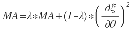
Rmsprop

算法是从

Rprop

算法中得到灵感的，它保留了对于每一个参数

θ

的平方梯度的平均移动，如下：



其中，

λ

是一个平均移动参数。

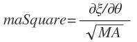
这时候，梯度已经被归一化了，如下：



之后，这个归一化的梯度被用于参数的更新。

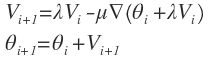
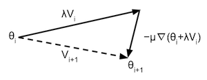
注意，这个梯度不是直接被使用在参数的更新上面，而是用在每个参数的速度参数（Vs）上面的更新。这个参数和这篇博客中的动量部分中的速度参数很像，但是在使用的方法上面又有一点差异。Nesterov 的加速梯度和一般的动量方法是不同的，主要体现在更新迭代方面。常规的动量算法在每一次迭代的开始就计算梯度，并且更新速度参数。但是 Nesterov 的加速梯度算法是根据较少速度来计算梯度的值，然后再更新速度，最后再根据局部梯度进行移动。这种处理方法有一个优点就是梯度在进行局部更新时将得到更多的信息，即使当前速度进行了一个错误的更新，该算法也能使梯度进行正确的计算。Nesterov 的更新可以如下计算：



其中，

∇(θ)

是一个在关于参数

θ

的局部梯度。比如，当前是第

i

次循环，那么式子可以被表示为如下图：



注意，我们不能保证一定会收敛到全局最小值，即

cost = 0

。因为如果你在参数更新的开始取的位置不是很好，那么最后的优化可能会取到局部最小值。而且训练过程对参数

lmbd

，

learning_rate

，

mementum_term

，

eps

都很敏感。你可以尝试一下以下代码，看看运行多久可以达到收敛。

# Set hyper-parameters
lmbd = 0.5  # Rmsprop lambda
learning_rate = 0.05  # Learning rate
momentum_term = 0.80  # Momentum term
eps = 1e-6  # Numerical stability term to prevent division by zero
mb_size = 100  # Size of the minibatches (number of samples)

# Create the network
nb_of_states = 3  # Number of states in the recurrent layer
RNN = RnnBinaryAdder(2, 1, nb_of_states, sequence_len)
# Set the initial parameters
nbParameters =  sum(1 for _ in RNN.get_params_iter())  # Number of parameters in the network
maSquare = [0.0 for _ in range(nbParameters)]  # Rmsprop moving average
Vs = [0.0 for _ in range(nbParameters)]  # Velocity

# Create a list of minibatch costs to be plotted
ls_of_costs = [RNN.cost(RNN.getOutput(X_train[0:100,:,:]), T_train[0:100,:,:])]
# Iterate over some iterations
for i in range(5):
# Iterate over all the minibatches
for mb in range(nb_train/mb_size):
X_mb = X_train[mb:mb+mb_size,:,:]  # Input minibatch
T_mb = T_train[mb:mb+mb_size,:,:]  # Target minibatch
V_tmp = [v * momentum_term for v in Vs]
# Update each parameters according to previous gradient
for pIdx, P in enumerate(RNN.get_params_iter()):
P += V_tmp[pIdx]
# Get gradients after following old velocity
backprop_grads = RNN.getParamGrads(X_mb, T_mb)  # Get the parameter gradients
# Update each parameter seperately
for pIdx, P in enumerate(RNN.get_params_iter()):
# Update the Rmsprop moving averages
maSquare[pIdx] = lmbd * maSquare[pIdx] + (1-lmbd) * backprop_grads[pIdx]**2
# Calculate the Rmsprop normalised gradient
pGradNorm = learning_rate * backprop_grads[pIdx] / np.sqrt(maSquare[pIdx] + eps)
# Update the momentum velocity
Vs[pIdx] = V_tmp[pIdx] - pGradNorm
P -= pGradNorm   # Update the parameter
ls_of_costs.append(RNN.cost(RNN.getOutput(X_mb), T_mb))  # Add cost to list to plot

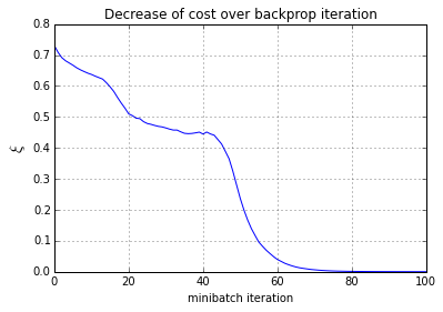
# Plot the cost over the iterations
plt.plot(ls_of_costs, 'b-')
plt.xlabel('minibatch iteration')
plt.ylabel('$\\xi$', fontsize=15)
plt.title('Decrease of cost over backprop iteration')
plt.grid()
plt.show()

测试网络

下面代码对我们上述设计的循环神经网络进行了二进制相加的测试，具体结果如下：

# Create test samples
nb_test = 5
Xtest, Ttest = create_dataset(nb_test, sequence_len)
# Push test data through network
Y = RNN.getBinaryOutput(Xtest)
Yf = RNN.getOutput(Xtest)

# Print out all test examples
for i in range(Xtest.shape[0]):
printSample(Xtest[i,:,0], Xtest[i,:,1], Ttest[i,:,:], Y[i,:,:])
print ''

x1: 0100010 34
x2: + 1100100 19
------- --
t: = 1010110 53
y: = 1010110

x1: 1010100 21
x2: + 1110100 23
------- --
t: = 0011010 44
y: = 0011010

x1: 1111010 47
x2: + 0000000 0
------- --
t: = 1111010 47
y: = 1111010

x1: 1000000 1
x2: + 1111110 63
------- --
t: = 0000001 64
y: = 0000001

x1: 1010100 21
x2: + 1010100 21
------- --
t: = 0101010 42
y: = 0101010

完整代码，点击这里