Andrew NG 机器学习 练习1-Linear Regression
2017-08-25 21:06
225 查看
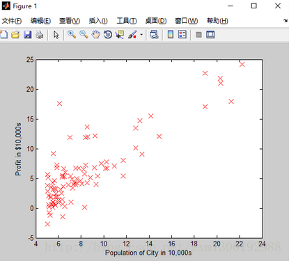
在本次练习中,需要实现一个单变量的线性回归。假设有一组历史数据<城市人口,开店利润>,现需要预测在哪个城市中开店利润比较好?
历史数据如下:第一列表示城市人口数,单位为万人;第二列表示利润,单位为10,000$
ex1data1.txt
6.1101,17.592
5.5277,9.1302
8.5186,13.662
7.0032,11.854
…
…
用Matlab画出的图形:首先加载数据,将data中的第一列数据保存到X中,将data中的所有行的第2列数据保存到y中
plotData.m代码如下:执行plot函数画图;xlabel、ylabel分别给X轴和Y轴标记提示信息。
画出来的图形如下:
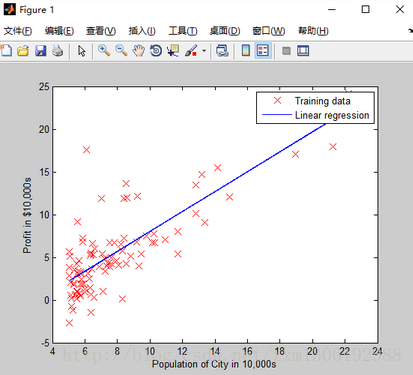
求得的线性回归模型如下图:
ex1data2.txt
The first column is the size of the house (in square feet),
the second column is the number of bedrooms,
and the third column is the price of the house.
2104,3,399900
1600,3,329900
2400,3,369000
1416,2,232000
…,…,…
…
标准化特征(Feature Normalization)
featureNormalize.m
代价函数和梯度下降函数,可以复用单变量线性回归实现,因为上述方法为向量化的矩阵操作,同样适用于多变量
computeCostMulti.m
gradientDescentMulti.m
使用正规方程方法,求参数
θ=(XTX)−1XTy
normalEqn.m

历史数据如下:第一列表示城市人口数,单位为万人;第二列表示利润,单位为10,000$
ex1data1.txt
6.1101,17.592
5.5277,9.1302
8.5186,13.662
7.0032,11.854
…
…
用Matlab画出的图形:首先加载数据,将data中的第一列数据保存到X中,将data中的所有行的第2列数据保存到y中
data = load('ex1data1.txt'); %读取以逗号分隔的数据
X = data(:, 1); y = data(:, 2); %将第一列放在X向量中%将第二列放在y向量中
m = length(y); %测试数据的个数

% Plot Data
% Note: You have to complete the code in plotData.m
plotData(X, y);
plotData.m代码如下:执行plot函数画图;xlabel、ylabel分别给X轴和Y轴标记提示信息。
function plotData(x, y)
%PLOTDATA Plots the data points x and y into a new figure
%   PLOTDATA(x,y) plots the data points and gives the figure axes labels of
%   population and profit.

figure; % open a new figure window

% ====================== YOUR CODE HERE ======================
% Instructions: Plot the training data into a figure using the
%               "figure" and "plot" commands. Set the axes labels using
%               the "xlabel" and "ylabel" commands. Assume the
%               population and revenue data have been passed in
%               as the x and y arguments of this function.
%
% Hint: You can use the 'rx' option with plot to have the markers
%       appear as red crosses. Furthermore, you can make the
%       markers larger by using plot(..., 'rx', 'MarkerSize', 10);

plot(x,y,'rx','MarkerSize',10); %plot the data, red颜色的X标记,标记的大小为 10
ylabel('Profit in $10,000s');
xlabel('Population of city in 10,000s');

% ============================================================

end
画出来的图形如下:
%% =================== Part 3: Cost and Gradient descent ===================

X = [ones(m, 1), data(:,1)]; % Add a column of ones to x
theta = zeros(2, 1); % initialize fitting parameters

% Some gradient descent settings
iterations = 1500;
alpha = 0.01; %learning rate

fprintf('\nTesting the cost function ...\n')
% compute and display initial cost
J = computeCost(X, y, theta);
fprintf('With theta = [0 ; 0]\nCost computed = %f\n', J);
fprintf('Expected cost value (approx) 32.07\n');

% further testing of the cost function
J = computeCost(X, y, [-1 ; 2]);
fprintf('\nWith theta = [-1 ; 2]\nCost computed = %f\n', J);
fprintf('Expected cost value (approx) 54.24\n');

fprintf('Program paused. Press enter to continue.\n');
pause;

fprintf('\nRunning Gradient Descent ...\n')
% run gradient descent
theta = gradientDescent(X, y, theta, alpha, iterations);

% print theta to screen
fprintf('Theta found by gradient descent:\n');
fprintf('%f\n', theta);
fprintf('Expected theta values (approx)\n');
fprintf(' -3.6303\n  1.1664\n\n');

% Plot the linear fit
hold on; % keep previous plot visible
plot(X(:,2), X*theta, '-')
legend('Training data', 'Linear regression')
hold off % don't overlay any more plots on this figure

% Predict values for population sizes of 35,000 and 70,000
predict1 = [1, 3.5] *theta;
fprintf('For population = 35,000, we predict a profit of %f\n',...
predict1*10000);
predict2 = [1, 7] * theta;
fprintf('For population = 70,000, we predict a profit of %f\n',...
predict2*10000);

fprintf('Program paused. Press enter to continue.\n');
pause;
function J = computeCost(X, y, theta) %COMPUTECOST Compute cost for linear regression % J = COMPUTECOST(X, y, theta) computes the cost of using theta as the % parameter for linear regression to fit the data points in X and y % Initialize some useful values m = length(y); % number of training examples % You need to return the following variables correctly J = 0; % ====================== YOUR CODE HERE ====================== % Instructions: Compute the cost of a particular choice of theta % You should set J to the cost. J=1/(2*m)*sum((X*theta-y).^2); % ========================================================================= end
function [theta, J_history] = gradientDescent(X, y, theta, alpha, num_iters)
%GRADIENTDESCENT Performs gradient descent to learn theta
%   theta = GRADIENTDESCENT(X, y, theta, alpha, num_iters) updates theta by
%   taking num_iters gradient steps with learning rate alpha

% Initialize some useful values
m = length(y); % number of training examples
J_history = zeros(num_iters, 1);

for iter = 1:num_iters

% ====================== YOUR CODE HERE ======================
% Instructions: Perform a single gradient step on the parameter vector
%               theta.
%
% Hint: While debugging, it can be useful to print out the values
%       of the cost function (computeCost) and gradient here.
%
theta=theta-(alpha/m)*X'*(X*theta-y);
% ============================================================

% Save the cost J in every iteration
J_history(iter) = computeCost(X, y, theta);

end

end
求得的线性回归模型如下图:
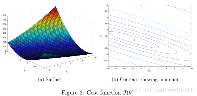
%% ============= Part 4: Visualizing J(theta_0, theta_1) =============
fprintf('Visualizing J(theta_0, theta_1) ...\n')

% Grid over which we will calculate J
theta0_vals = linspace(-10, 10, 100); %线性间隔向量,在-10和10之间100个点
theta1_vals = linspace(-1, 4, 100);

% initialize J_vals to a matrix of 0's
J_vals = zeros(length(theta0_vals), length(theta1_vals));

% Fill out J_vals
for i = 1:length(theta0_vals)
for j = 1:length(theta1_vals)
t = [theta0_vals(i); theta1_vals(j)];
J_vals(i,j) = computeCost(X, y, t);
end
end

% Because of the way meshgrids work in the surf command, we need to
% transpose J_vals before calling surf, or else the axes will be flipped
J_vals = J_vals';
% Surface plot
figure;
surf(theta0_vals, theta1_vals, J_vals)
xlabel('\theta_0'); ylabel('\theta_1');

% Contour plot
figure;
% Plot J_vals as 15 contours spaced logarithmically between 0.01 and 100
contour(theta0_vals, theta1_vals, J_vals, logspace(-2, 3, 20)) %绘制等高线,生成10的-2次方到10的3次方之间的按对数等分的n个元素的行向量
xlabel('\theta_0'); ylabel('\theta_1');
hold on;
plot(theta(1), theta(2), 'rx', 'MarkerSize', 10, 'LineWidth', 2);
多变量的线性回归(Linear regression with multiple variables)
Suppose you are selling your house and you want to know what a good market price would be. One way to do this is to first collect information on recent houses sold and make a model of housing prices.ex1data2.txt
The first column is the size of the house (in square feet),
the second column is the number of bedrooms,
and the third column is the price of the house.
2104,3,399900
1600,3,329900
2400,3,369000
1416,2,232000
…,…,…
…
标准化特征(Feature Normalization)
%% ================ Part 1: Feature Normalization ================

%% Clear and Close Figures
clear ; close all; clc

fprintf('Loading data ...\n');

%% Load Data
data = load('ex1data2.txt');
X = data(:, 1:2);
y = data(:, 3);
m = length(y);

% Print out some data points
fprintf('First 10 examples from the dataset: \n');
fprintf(' x = [%.0f %.0f], y = %.0f \n', [X(1:10,:) y(1:10,:)]');

fprintf('Program paused. Press enter to continue.\n');
pause;

% Scale features and set them to zero mean
fprintf('Normalizing Features ...\n');

[X,mu,sigma] = featureNormalize(X);

% Add intercept term to X
X = [ones(m, 1) X]
featureNormalize.m
function [X_norm, mu, sigma] = featureNormalize(X)
%FEATURENORMALIZE Normalizes the features in X
%   FEATURENORMALIZE(X) returns a normalized version of X where
%   the mean value of each feature is 0 and the standard deviation
%   is 1. This is often a good preprocessing step to do when
%   working with learning algorithms.

% You need to set these values correctly
X_norm = X;
mu = zeros(1, size(X, 2));
sigma = zeros(1, size(X, 2));

% ====================== YOUR CODE HERE ======================
% Instructions: First, for each feature dimension, compute the mean
%               of the feature and subtract it from the dataset,
%               storing the mean value in mu. Next, compute the
%               standard deviation of each feature and divide
%               each feature by it's standard deviation, storing
%               the standard deviation in sigma.
%
%               Note that X is a matrix where each column is a
%               feature and each row is an example. You need
%               to perform the normalization separately for
%               each feature.
%
% Hint: You might find the 'mean' and 'std' functions useful.
%

%方法1:按行求(提交有错)
% mu=mean(X);
% sigma=[std(X(:,1)),std(X(:,2))];
% for i=1:size(X,1),
%     X_norm(i,:)=(X(i,:)-mu)./sigma;
% end;

%方法2:按列求
% for iter = 1:size(X, 2) %分两列分别求
%     mu(1, iter) = mean(X(:, iter)); %第1或2列的均值
%     sigma(1, iter) = std(X(:, iter)); %第1或2列的标准差
%     X_norm(:, iter) = (X_norm(:, iter) - mu(1, iter)) ./ sigma(1, iter);

%方法3:向量化一起求
len = length(X);
mu = mean(X);
sigma = std(X);
X_norm = (X - ones(len, 1) * mu) ./ (ones(len, 1) * sigma);

% ============================================================

end
代价函数和梯度下降函数,可以复用单变量线性回归实现,因为上述方法为向量化的矩阵操作,同样适用于多变量
computeCostMulti.m
gradientDescentMulti.m
%% ================ Part 2: Gradient Descent ================

% ====================== YOUR CODE HERE ======================
% Instructions: We have provided you with the following starter
%               code that runs gradient descent with a particular
%               learning rate (alpha).
%
%               Your task is to first make sure that your functions -
%               computeCost and gradientDescent already work with
%               this starter code and support multiple variables.
%
%               After that, try running gradient descent with
%               different values of alpha and see which one gives
%               you the best result.
%
%               Finally, you should complete the code at the end
%               to predict the price of a 1650 sq-ft, 3 br house.
%
% Hint: By using the 'hold on' command, you can plot multiple
%       graphs on the same figure.
%
% Hint: At prediction, make sure you do the same feature normalization.
%

fprintf('Running gradient descent ...\n');

% Choose some alpha value
alpha = 0.01;
num_iters = 800;

% Init Theta and Run Gradient Descent
theta = zeros(3, 1);
[theta, J_history] = gradientDescentMulti(X, y, theta, alpha, num_iters);

% Plot the convergence graph
figure;
plot(1:numel(J_history), J_history, '-b', 'LineWidth', 2);
xlabel('Number of iterations');
ylabel('Cost J');

% Display gradient descent's result
fprintf('Theta computed from gradient descent: \n');
fprintf(' %f \n', theta);
fprintf('\n');

% Estimate the price of a 1650 sq-ft, 3 br house
% ====================== YOUR CODE HERE ======================
% Recall that the first column of X is all-ones. Thus, it does
% not need to be normalized.
X_test=[1650 3];
[X_test,mu,sigma] =featureNormalize2(X_test,mu,sigma);%使用样本数据的均值,和标准差,进行归一化
price = [1 X_test]*theta;

% ============================================================

fprintf(['Predicted price of a 1650 sq-ft, 3 br house ' ...
'(using gradient descent):\n $%f\n'], price);

fprintf('Program paused. Press enter to continue.\n');
pause;

%% ================ Part 3: Normal Equations ================

fprintf('Solving with normal equations...\n');

% ====================== YOUR CODE HERE ======================
% Instructions: The following code computes the closed form
%               solution for linear regression using the normal
%               equations. You should complete the code in
%               normalEqn.m
%
%               After doing so, you should complete this code
%               to predict the price of a 1650 sq-ft, 3 br house.
%

%% Load Data
data = csvread('ex1data2.txt');
X = data(:, 1:2);
y = data(:, 3);
m = length(y);

% Add intercept term to X
X = [ones(m, 1) X];

% Calculate the parameters from the normal equation
theta = normalEqn(X, y);%使用正规方程的数据,不需要归一化

% Display normal equation's result
fprintf('Theta computed from the normal equations: \n');
fprintf(' %f \n', theta);
fprintf('\n');

% Estimate the price of a 1650 sq-ft, 3 br house
% ====================== YOUR CODE HERE ======================
X_test=[1650 3];
price = [1 X_test]*theta;

% ============================================================

fprintf(['Predicted price of a 1650 sq-ft, 3 br house ' ...
'(using normal equations):\n $%f\n'], price);
使用正规方程方法,求参数
θ=(XTX)−1XTy
normalEqn.m
function [theta] = normalEqn(X, y)
%NORMALEQN Computes the closed-form solution to linear regression
%   NORMALEQN(X,y) computes the closed-form solution to linear
%   regression using the normal equations.

theta = zeros(size(X, 2), 1);

% ====================== YOUR CODE HERE ======================
% Instructions: Complete the code to compute the closed form solution
%               to linear regression and put the result in theta.
%

% ---------------------- Sample Solution ----------------------
theta = pinv(X' * X) * X' * y

% ============================================================

end

相关文章推荐
- Andrew NG 机器学习 练习6-Support Vector Machines
- Andrew NG 机器学习 练习2-Logistic Regression
- Andrew NG 机器学习 练习5-Regularized Linear Regression and Bias/Variance
- Andrew NG 机器学习 练习3-Multiclass Classification and Neural Networks
- Andrew NG 机器学习 练习8-Anomaly Detection and Recommender Systems
- Andrew NG 机器学习 练习7-K-means Clustering and Principal Component Analysis
- Andrew NG 机器学习 练习4-Neural Networks Learning
- Andrew Ng coursera上的《机器学习》ex6
- 斯坦福大学Andrew Ng教授主讲的《机器学习》公开课观后感
- 看完吴恩达(Andrew Ng)机器学习视频的感受
- COURSERA 机器学习课笔记(by Prof. Andrew Ng)学习笔记(一)
- Coursera-吴恩达-机器学习-(编程练习5)Bias and Variance(对应第6周课程)
- 斯坦福大学Andrew Ng教授主讲的《机器学习》公开课观后感
- 【机器学习】UFLDL练习1
- 多类别分类-机器学习(machine learning)笔记(Andrew Ng)
- 机器学习练习之正则化
- 收藏!斯坦福Andrew Ng教授“机器学习”26篇教程全译
- 周志华《机器学习》课后习题解答系列(四):Ch3.4 - 交叉验证法练习
- 斯坦福大学公开课 :机器学习课程(Andrew Ng)——10、无监督学习:Mixture of Gaussians and the EM Algorithm
- 斯坦福大学公开课 :机器学习课程(Andrew Ng)——11、无监督学习:the derivation of EM Algorithm