TensorFlow搭建CNN卷积神经网络

TensorFlow搭建CNN卷积神经网络

该教程采用TernsorFlow搭建CNN卷积神经网络，并利用MNIST数据集进行数字的手写识别

数据结构

mnist原始图片输入，原始图片的尺寸为28×28，导入后会自动展开为28×28=784的list

tensor : shape=[784]

卷积层输入input_image: shape=[batch, height, width, channels]

bacth : 取样数

height, width : 图片的尺寸

channels : 图片的深度；如果是灰度图像，则为1，rgb图像，则为3

卷积核filter: shape=[height, width, in_channels, out_channels]

height, width: 图片的尺寸

in_channels: 图片的深度

out_channels: 卷积核的数量

对于in_channels，灰度图为1，rgb图为3

函数

TensorFlow自带的CNN操作函数

卷积函数[tf.nn.conv2d(x, filter, strides=[1,1,1,1], padding=’SAME’)]

x: 卷积层输入 shape=[batch, height, width, channels]

filter: 卷积核 shape=[height, width, in_channels, out_channels]

stride: 卷积步长 shape=[batch_stride, height_stride, width_stride, channels_stride]

padding: 控制卷积核处理边界的策略

stride表示卷积核filter对应了input_image各维度下移动的步长；第一个参数对应input_image的batch方向上的移动步长，第二、三参数对应高宽方向上的步长，决定了卷积后图像的尺寸，最后一个参数对应channels方向上的步长

padding=’SAME’表示给图像边界加上padding，让filter卷积后的图像尺寸与原图相同；’VALID’表示卷积后imgaeHeight_aterFiltered=imageHeight_inital-filterHeight+strideHeight，宽同理

池化函数tf.nn.max_pool(x, k_size=[1,2,2,1], strides=[1,2,2,1], padding=’SAME’)

x: 池化输入input_image: shape=[batch, height, width, channels]

ksize: 池化窗口的尺寸

strides: 池化步长

padding: 处理边界策略

池化输入，tensor的shape同input_image, 一般为卷积后图像feature_map

ksize对应输入图像各维度的池化尺寸；第一个参数对应batch方向上的池化尺寸，第二、三参数对应图像高宽上的池化尺寸，第四个参数对应channels方向上的池化尺寸，一般不在batch和channel方向上做池化，因此通常为[1,height,width,1]

strides与padding同卷积函数tf.nn.conv2d()

为了方便后续搭建，需要自己定义一些函数

卷积核filter初始化weight_variable(shape)

def weight_variable(shape):
initial=tf.truncated_normal(shape, mean=0.0, stddev=0.1)
return tf.Variable(inital)

对于CNN来说，weight实际上就是卷积核filter，因此shape应该与tf.nn.conv2d中filter的shape一致，即shape=[height, width, in_channels, out_channels]

tf.truncated_normal()表示截断正态分布，即保留[mean-2×stddev,mean+2×stddev]范围内的随机数，mean表示平均数，stddev为方差

偏置初始化bias_variable(shape)

def bias_variable(shape):
initial=tf.constant(0,1,shape=shape)
return tf.Vatiable(initial)

针对tensorFlow函数更详细的使用，参见tensorFlow常用函数汇总

思路

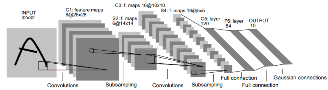
详细CNN过程

MNIST数据导入

代码这一行就是用于下载mnist数据，实际操作过程往往会出现socket error，因此需要事先下载好

from tensorflow.examples.tutorials.mnist import input_data

在程序的文件夹下建立MNIST_data文件夹，在执行完上述代码后，会自动生成该文件夹

进入MNIST_data文件后，从github上直接下载数据集合

cd MNIST_data
git clone https://github.com/HIPS/hypergrad.git #下载完成后，将下载文件中data/mnist下所有数据copy进MNIST_data中即可

完整代码

import tensorflow as tf
from tensorflow.examples.tutorials.mnist import input_data

#获取mnist训练集
mnist = input_data.read_data_sets("MNIST_data/", one_hot=True)

#交互式session
sess = tf.InteractiveSession()

#已将32×32的图片展开成行向量，None代表该维度上数量不确定，程序中指的是取样的图像数量不确定
x=tf.placeholder(tf.float32, shape=[None,784])
#图片的标签
y_label=tf.placeholder(tf.float32, shape=[None,10])
-------------------------------------------------------------------------
#第一层网络
#reshape()将按照设定的shape=[-1,28,28,1]对x:shape=[None,784]的结构进行重新构建
#参数-1代表该维度上数量不确定，由系统自动计算
x_image = tf.reshape(x, shape=[-1,28,28,1])
#32个卷积核，卷积核大小5×5
W_conv1 = weight_variable([5,5,1,32])
#32个前置，对应32个卷积核输出
b_conv1 = bias_varibale([32])

#卷积操作
layer_conv1 = tf.nn.relu(conv2d(x_image, W_conv1) + b_conv1)
#池化操作
layer_pool1 = tf.nn.max_pool(layer_conv1)
-------------------------------------------------------------------------
#第二层网络
#64个卷积核，卷积核大小5×5，32个channel
W_conv2 = weight_variable([5,5,32,64])
#64个前置，对应64个卷积核输出
b_conv2 = bias_varibale([64])

#卷积操作
layer_conv2 = tf.nn.relu(conv2d(layer_pool1, W_conv2) + b_conv2)
#池化操作
layer_pool2 = tf.nn.max_pool(layer_conv2)
-------------------------------------------------------------------------
#full-connected网络
#图片尺寸变化28×28-->14×14-->7×7
#该层设定1024个神经元
layer_pool2_flat = tf.reshape(layer_pool2,[-1,7*7*64])

W_fc1 = weight_variable([7*7*64,1024])
b_fc1 = bias_variable([1024])

h_fc1 = tf.nn.relu(tf.matmul(layer_pool2_flat, W_fc1) + b_fc1)
-------------------------------------------------------------------------
#droput网络
keep_prob = tf.placeholder(tf.float32)
h_fc1_drop = tf.nn.dropout(h_fc1, keep_prob)
-------------------------------------------------------------------------
#输出层
W_fc2 = weight_variable([1024,10])
b_fc2 = bias_variable([10])

y_conv = tf.nn.softmax(tf.matmul(h_fc1_drop,W_fc2)+b_fc2)
-------------------------------------------------------------------------
#loss-function
cross_entropy = -tf.reduce_sum(y_lable*tf.log(y_conv))
#梯度下降
train = tf.train.GradientDescentOptimizer(0.01).minimize(cross_entropy)
#tf.argmax(x,1)表示从x的第二维度选取最大值
correct_prediction = tf.equal(tf.argmax(y_conv,1), tf.argmax(y_lable,1))
accuracy = tf.reduce_mean(tf.cast(correct_prediction,tf.float32))
sess.run(tf.global_variables_initializer())
-------------------------------------------------------------------------
#训练train
#训练3000次
for i in range(3000)
#每次选取50训练集
batch = mnist.train.next_batch(50)

if i%100 == 0:
train_accuracy = accuracy.eval(feed_dict={x:batch[0], y_labe: batch[1], keep_prob: 1.0})
print ("step %d, training accuracy %g"%(i, train_accuracy))

train.run(feed_dict={x: batch[0], y_label: batch[1], keep_prob: 0.5})
print ("test accuracy %g"%accuracy.eval(feed_dict={x: mnist.test.images, y_label: mnist.test.labels, keep_prob: 1.0}))

详细代码