机器学习-->检测异常样本方法总结
2017-08-18 16:17
447 查看
数据预处理的好坏,很大程度上决定了模型分析结果的好坏。其中,异常值(outliers)检测是整个数据预处理过程中,十分重要的一环。方法也是多种多样。
由于异常值检验,和去重、缺失值处理不同,它带有一定的主观性。在实际业务场景中,我们要根据具体的业务逻辑来判别哪些样本是离群点。
下面总结下我平时经常用到的异常样本检测方法,可能总结的不全。
,那么可以计算出这 n 个点的均值

和方差

。均值和方差分别被定义为:

在正态分布的假设下,区域

包含了99.7% 的数据,如果某个值距离分布的均值
超过了

,那么这个值就可以被简单的标记为一个异常点(outlier)。
,即有m个样本,n个特征。那么可以计算每个维度的均值和方差

。那么可以计算每个特征的平均值和方差:
在正态分布的假设下,如果有一个新的数据

,可以计算概率

如下:
根据概率值的大小就可以判断 x 是否属于异常值。

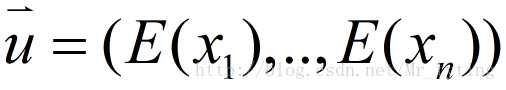
,可以计算 n 维的均值向量:
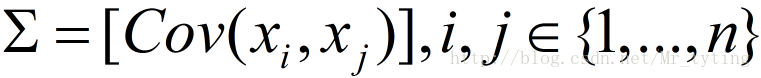
和 n*n 的协方差矩阵:
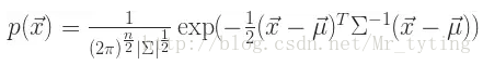
如果有一个新的数据
,可以计算:

是均值向量,那么对于数据集 D 中的其他对象 a,从 a 到
的 Mahalanobis 距离是:

其中 S 是协方差矩阵。
在这里,

是数值,可以对这个数值进行排序,如果数值过大,那么就可以认为点 a 是离群点。或者对一元实数集合

进行离群点检测,如果
被检测为异常点,那么就认为 a 在多维的数据集合 D 中就是离群点。
特征是二维时,用马氏距离检查异常值:

很好的识别出两个异常值。
当特征是三维时,用马氏距离检查异常值:
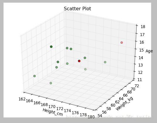
注意:当你的数据表现出非线性关系关系时,你可要谨慎使用该方法了,马氏距离仅仅把他们作为线性关系处理。例如上面的身高和体重的关系,按常识,身高和体重必然存在线性关系所以马氏距离能很好的检测到异常值,但是是如果是非线性关系就得谨慎使用马氏距离了。
使用
在正态分布的假设下,

统计量可以用来检测多元离群点。对于某个对象 a,
统计量是:

其中,

是a在第 i 维上的取值,

是所有对象在第 i 维的均值,n 是维度。如果对象 a 的
统计量很大,那么该对象就可以认为是离群点。
PCA原理请看我的另外一篇博文:PCA
怎么来切这个数据空间是iForest的设计核心思想。由于切割是随机的,所以需要用ensemble的方法来得到一个收敛值,即反复从头开始切,然后平均每次切的结果。iForest 由t个iTree(Isolation Tree)孤立树 组成,每个iTree是一个二叉树结构,其实现步骤如下:
从训练数据中随机选择Ψ个点样本点作为subsample,放入树的根节点。
随机指定一个维度(attribute),在当前节点数据中随机产生一个切割点p——切割点产生于当前节点数据中指定维度的最大值和最小值之间。
以此切割点生成了一个超平面,然后将当前节点数据空间划分为2个子空间:把指定维度里小于p的数据放在当前节点的左孩子,把大于等于p的数据放在当前节点的右孩子。
在孩子节点中递归步骤2和3,不断构造新的孩子节点,直到 孩子节点中只有一个数据(无法再继续切割) 或 孩子节点已到达限定高度 。
然后在生成的iForest内计算:
计算iTree中样本x从根到叶子的长度f(x)。
计算iForest中f(x)的总和F(x) 。
异常检测:若样本x为异常值,它应在大多 数iTree中很快从根到达叶子,即F(x)较小。
sklearn中的iForest:
sklearn.ensemble.IsolationForest(n_estimators=100, max_samples=’auto’, contamination=0.1, max_features=1.0, bootstrap=False, n_jobs=1, random_state=None, verbose=0)
具体参数解释请看 sklearn.ensemble.IsolationForest
由画出的结果可知,显然黑色样本离群较大,应该属于异常值,决策边界也很好的将其划分出来了。那我现在把识别出来的异常值去掉看看效果如何?

显然去掉的样本的确为异常值。
实际上,从k个最近的邻居获得局部密度。观察的LOF得分等于他的k个最近邻居的平均局部密度与其本地密度的比值:正常样本预计具有与其邻居类似的局部密度,而异常样本的局部密度预计要比其邻居的局部密度小得多。
邻居的数量k的选择是个需要考虑的问题,通常k = 20时总体上很好地工作。当异常值的比例很高时k应该更大。
LOF算法的优点在于它考虑了数据集的本地和全局属性:即使在异常样本具有不同基础密度的数据集中,它也能很好地执行。问题不在于,样本是如何孤立的,而是与周围邻居的隔离程度。
sklearn中LOF函数详情请看sklearn.neighbors.LocalOutlierFactor
显然在这个数据集中很好的去除了异常样本。
上述代码中,我们为DBSCAN选用了六组参数,画出在这六组参数下,对样本集聚类情况,并且识别出离群样本。离群样本为下图中的黑色原点。

在不同的参数下识别离群样本准备程度不一样。
那我们现在去掉这些识别出的黑色样本看看效果如何?

感觉清爽多了!并且有上图可以看出参数选择(0.2,15)时,聚类效果最好。
由于异常值检验,和去重、缺失值处理不同,它带有一定的主观性。在实际业务场景中,我们要根据具体的业务逻辑来判别哪些样本是离群点。
下面总结下我平时经常用到的异常样本检测方法,可能总结的不全。
可视化的方法
对于样本集某一个特征而言,可以直接画出这个样本集在这个特征上值的分布情况,如果有一些数据明显过高或者过低,则可以视其为异常样本去掉即可。概率统计的方法
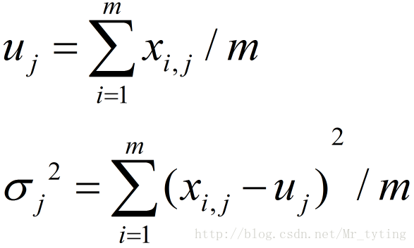
基于正态分布的一元离群点检测方法
假设有 n 个点,那么可以计算出这 n 个点的均值
和方差
。均值和方差分别被定义为:
在正态分布的假设下,区域
包含了99.7% 的数据,如果某个值距离分布的均值
超过了
,那么这个值就可以被简单的标记为一个异常点(outlier)。
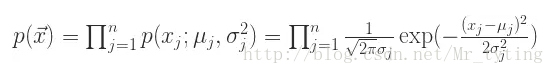
基于一元正态分布的离群点检测方法
假设 n 维的数据集合形如,即有m个样本,n个特征。那么可以计算每个维度的均值和方差
。那么可以计算每个特征的平均值和方差:
在正态分布的假设下,如果有一个新的数据
,可以计算概率
如下:
根据概率值的大小就可以判断 x 是否属于异常值。
多元高斯分布的异常点检测
假设 n 维的数据集合,可以计算 n 维的均值向量:
和 n*n 的协方差矩阵:
如果有一个新的数据
,可以计算:
使用 Mahalanobis 距离检测多元离群点
对于一个多维的数据集合 D,假设是均值向量,那么对于数据集 D 中的其他对象 a,从 a 到
的 Mahalanobis 距离是:
其中 S 是协方差矩阵。
在这里,
是数值,可以对这个数值进行排序,如果数值过大,那么就可以认为点 a 是离群点。或者对一元实数集合
进行离群点检测,如果
被检测为异常点,那么就认为 a 在多维的数据集合 D 中就是离群点。
特征是二维时,用马氏距离检查异常值:
#coding:utf-8

from numpy import float64
from matplotlib import pyplot as plt
import pandas as pd
import numpy as np
from scipy.spatial import distance
from pandas import Series

Height_cm = np.array([164, 167, 168, 169, 169, 170, 170, 170, 171, 172, 172, 173, 173, 175, 176, 178], dtype=float64)
Weight_kg = np.array([54,  57,  58,  60,  61,  60,  61,  62,  62,  64,  62,  62,  64,  56,  66,  70], dtype=float64)
hw = {'Height_cm': Height_cm, 'Weight_kg': Weight_kg}
hw = pd.DataFrame(hw)

n_outliers = 2##这里只检测两个异常值
## 计算每个样本的马氏距离,并且从大到小排序,越大则越有可能是离群点,返回其索引
m_dist_order = Series([float(distance.mahalanobis(hw.iloc[i], hw.mean(), np.mat(hw.cov().as_matrix()).I) ** 2)
for i in range(len(hw))]).sort_values(ascending=False).index.tolist()

is_outlier = [False, ] * 16 ##返回长度为16的全FALSE的列表
for i in range(n_outliers):## n_outliers = 2,找出马氏距离最大的两个样本,标记为True,为离群点
is_outlier[m_dist_order[i]] = True

color = ['g', 'black']
pch = [1 if is_outlier[i] == True else 0 for i in range(len(is_outlier))]
cValue = [color[is_outlier[i]] for i in range(len(is_outlier))]
fig = plt.figure()
plt.title('Scatter Plot')
plt.xlabel('Height_cm')
plt.ylabel('Weight_kg')
plt.scatter(hw['Height_cm'], hw['Weight_kg'], s=40, c=cValue)
plt.show()
很好的识别出两个异常值。
当特征是三维时,用马氏距离检查异常值:
#coding:utf-8

import pandas as pd
from sklearn import preprocessing
import numpy as np
from numpy import float64
from matplotlib import pyplot as plt
from scipy.spatial import distance
from pandas import Series
import mpl_toolkits.mplot3d

Height_cm = np.array([164, 167, 168, 168, 169, 169, 169, 170, 172, 173, 175, 176, 178], dtype=float64)
Weight_kg = np.array([55,  57,  58,  56,  57,  61,  61,  61,  64,  62,  56,  66,  70], dtype=float64)
Age = np.array([13,  12,  14,  17,  15,  14,  16,  16,  13,  15,  16,  14,  16], dtype=float64)
hw = {'Height_cm': Height_cm, 'Weight_kg': Weight_kg, 'Age': Age}
hw = pd.DataFrame(hw)

n_outliers = 2

m_dist_order =  Series([float(distance.mahalanobis(hw.iloc[i], hw.mean(), np.mat(hw.cov().as_matrix()).I) ** 2)
for i in range(len(hw))]).sort_values(ascending=False).index.tolist()
is_outlier = [False, ] * 13
for i in range(n_outliers):
is_outlier[m_dist_order[i]] = True
# print is_outlier

color = ['g', 'r']
pch = [1 if is_outlier[i] == True else 0 for i in range(len(is_outlier))]
cValue = [color[is_outlier[i]] for i in range(len(is_outlier))]
# print cValue

fig = plt.figure()
ax1 = plt.subplot(111, projection='3d')
ax1.set_title('Scatter Plot')
ax1.set_xlabel('Height_cm')
ax1.set_ylabel('Weight_kg')
ax1.set_zlabel('Age')
ax1.scatter(hw['Height_cm'], hw['Weight_kg'], hw['Age'],  s=40, c=cValue)
plt.show()

##除去20%的异常样本,输出剩余80%的样本
percentage_to_remove = 20#除去20%的异常样本
number_to_remove = round(len(hw) * percentage_to_remove / 100)   # 四舍五入取整
rows_to_keep_index = m_dist_order[int(number_to_remove): ]
my_dataframe = hw.loc[rows_to_keep_index]
print my_dataframe注意:当你的数据表现出非线性关系关系时,你可要谨慎使用该方法了,马氏距离仅仅把他们作为线性关系处理。例如上面的身高和体重的关系,按常识,身高和体重必然存在线性关系所以马氏距离能很好的检测到异常值,但是是如果是非线性关系就得谨慎使用马氏距离了。
使用
统计量检测多元离群点
在正态分布的假设下,统计量可以用来检测多元离群点。对于某个对象 a,
统计量是:
其中,
是a在第 i 维上的取值,
是所有对象在第 i 维的均值,n 是维度。如果对象 a 的
统计量很大,那么该对象就可以认为是离群点。
PCA除去异常值
PCA对高维数据进行降维,其中降维是目的,最大方差是手段。其实就是保留效果最好的一个或最好的前几个相互正交的投影方向,使得样本值投影以后方差最大。这种投影可以理解对特征的重构或者是组合,其降维的结果往往是去除了异常值。PCA原理请看我的另外一篇博文:PCA
iForest (Isolation Forest)孤立森林 异常检测
iForest属于Non-parametric和unsupervised的方法,即不用定义数学模型也不需要有标记的训练。对于如何查找哪些点是否容易被孤立(isolated),iForest使用了一套非常高效的策略。假设我们用一个随机超平面来切割(split)数据空间(data space), 切一次可以生成两个子空间(想象拿刀切蛋糕一分为二)。之后我们再继续用一个随机超平面来切割每个子空间,循环下去,直到每子空间里面只有一个数据点为止。直观上来讲,我们可以发现那些密度很高的簇是可以被切很多次才会停止切割,但是那些密度很低的点很容易很早的就停到一个子空间了。怎么来切这个数据空间是iForest的设计核心思想。由于切割是随机的,所以需要用ensemble的方法来得到一个收敛值,即反复从头开始切,然后平均每次切的结果。iForest 由t个iTree(Isolation Tree)孤立树 组成,每个iTree是一个二叉树结构,其实现步骤如下:
从训练数据中随机选择Ψ个点样本点作为subsample,放入树的根节点。
随机指定一个维度(attribute),在当前节点数据中随机产生一个切割点p——切割点产生于当前节点数据中指定维度的最大值和最小值之间。
以此切割点生成了一个超平面,然后将当前节点数据空间划分为2个子空间:把指定维度里小于p的数据放在当前节点的左孩子,把大于等于p的数据放在当前节点的右孩子。
在孩子节点中递归步骤2和3,不断构造新的孩子节点,直到 孩子节点中只有一个数据(无法再继续切割) 或 孩子节点已到达限定高度 。
然后在生成的iForest内计算:
计算iTree中样本x从根到叶子的长度f(x)。
计算iForest中f(x)的总和F(x) 。
异常检测:若样本x为异常值,它应在大多 数iTree中很快从根到达叶子,即F(x)较小。
sklearn中的iForest:
sklearn.ensemble.IsolationForest(n_estimators=100, max_samples=’auto’, contamination=0.1, max_features=1.0, bootstrap=False, n_jobs=1, random_state=None, verbose=0)
具体参数解释请看 sklearn.ensemble.IsolationForest
print(__doc__)
import numpy as np
import matplotlib.pyplot as plt
from sklearn.ensemble import IsolationForest
rng = np.random.RandomState(42)
# Generate train data
X = 0.3 * rng.randn(100, 2)
X_train = np.r_[X + 2, X - 2]##按行堆叠,shape(200,2)
# Generate some regular novel observations
X = 0.3 * rng.randn(20, 2)
X_test = np.r_[X + 2, X - 2]##按行堆叠,shape(40,2)
# Generate some abnormal novel observations
X_outliers = rng.uniform(low=-4, high=4, size=(20, 2))##shape(20,2)
# fit the model
clf = IsolationForest(max_samples=100, random_state=rng)
clf.fit(X_train)## 训练出一个iForest,iForest为无监督的方法,但是也不能直接对无标记样本集预测,可以先fit无标记样本集,然后在predict
y_pred_train = clf.predict(X_train)
y_pred_test = clf.predict(X_test)
y_pred_outliers = clf.predict(X_outliers)
# plot the line, the samples, and the nearest vectors to the plane
xx, yy = np.meshgrid(np.linspace(-5, 5, 50), np.linspace(-5, 5, 50))
Z = clf.decision_function(np.c_[xx.ravel(), yy.ravel()])##按列堆叠shape(100,2),并且得出决策边界
Z = Z.reshape(xx.shape)
plt.title("IsolationForest")
plt.contourf(xx, yy, Z, cmap=plt.cm.Blues_r)##画出决策边界,不同的区域颜色不同
b1 = plt.scatter(X_train[:, 0], X_train[:, 1], c='white',
s=20, edgecolor='k')
b2 = plt.scatter(X_test[:, 0], X_test[:, 1], c='green',
s=20, edgecolor='k')
c = plt.scatter(X_outliers[:, 0], X_outliers[:, 1], c='red',
s=20, edgecolor='k')
plt.axis('tight')
plt.xlim((-5, 5))
plt.ylim((-5, 5))
plt.legend([b1, b2, c],
["training observations",
"new regular observations", "new abnormal observations"],
loc="upper left")
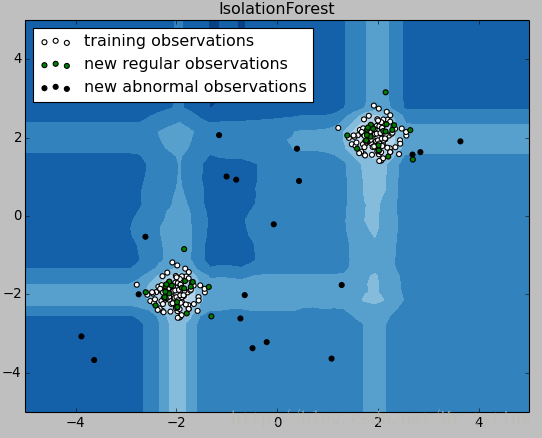
plt.show()由画出的结果可知,显然黑色样本离群较大,应该属于异常值,决策边界也很好的将其划分出来了。那我现在把识别出来的异常值去掉看看效果如何?
import numpy as np
import matplotlib.pyplot as plt
from sklearn.ensemble import IsolationForest

rng = np.random.RandomState(42)

# Generate train data
X = 0.3 * rng.randn(100, 2)
X_train = np.r_[X + 2, X - 2]
# Generate some regular novel observations
X = 0.3 * rng.randn(20, 2)
X_test = np.r_[X + 2, X - 2]
print X_test.shape
# Generate some abnormal novel observations
X_outliers = rng.uniform(low=-4, high=4, size=(20, 2))
print X_outliers.shape

# fit the model
clf = IsolationForest(max_samples=100, random_state=rng)
clf.fit(X_train)
y_pred_train = clf.predict(X_train)## 对样本的预测结果为1则说明为正常值,为-1表示为异常值

train_index=[]
for i,j in enumerate(y_pred_train):
if j==1:
train_index.append(i)## 获取所有正常值的索引

test_index=[]
y_pred_test = clf.predict(X_test)
for i,j in enumerate(y_pred_test):
if j==1:
test_index.append(i)

y_pred_outliers = clf.predict(X_outliers)
outliers_index=[]
for i,j in enumerate(y_pred_outliers):
if j==1:
outliers_index.append(i)

new_x_train=X_train[train_index]##将所有预测为正常样本重新组成新的样本集
new_x_test=X_test[test_index]
new_x_outliers=X_outliers[outliers_index]

# plot the line, the samples, and the nearest vectors to the plane
xx, yy = np.meshgrid(np.linspace(-5, 5, 50), np.linspace(-5, 5, 50))
Z = clf.decision_function(np.c_[xx.ravel(), yy.ravel()])
Z = Z.reshape(xx.shape)

plt.title("IsolationForest")
plt.contourf(xx, yy, Z, cmap=plt.cm.Blues_r)

## 画出各个样本集的正常值分布情况
b1 = plt.scatter(new_x_train[:, 0], new_x_train[:, 1], c='white',
s=20, edgecolor='k')
b2 = plt.scatter(new_x_test[:, 0], new_x_test[:, 1], c='green',
s=20, edgecolor='k')
c = plt.scatter(new_x_outliers[:, 0], new_x_outliers[:, 1], c='black',
s=20, edgecolor='k')
plt.axis('tight')
plt.xlim((-5, 5))
plt.ylim((-5, 5))
plt.legend([b1, b2, c],
["training observations",
"new regular observations", "new abnormal observations"],
loc="upper left")
plt.show()
显然去掉的样本的确为异常值。
Local Outlier Factor
neighbors.LocalOutlierFactor(LOF)算法用来计算观测样本异常程度的分数(称为局部离群因子)。是一种无监督方法。它测量给定数据点相对于其邻居的局部密度 偏差。这个算法就是检测那些周围密度比较低的样本,然后将他们标记为离群点。实际上,从k个最近的邻居获得局部密度。观察的LOF得分等于他的k个最近邻居的平均局部密度与其本地密度的比值:正常样本预计具有与其邻居类似的局部密度,而异常样本的局部密度预计要比其邻居的局部密度小得多。
邻居的数量k的选择是个需要考虑的问题,通常k = 20时总体上很好地工作。当异常值的比例很高时k应该更大。
LOF算法的优点在于它考虑了数据集的本地和全局属性:即使在异常样本具有不同基础密度的数据集中,它也能很好地执行。问题不在于,样本是如何孤立的,而是与周围邻居的隔离程度。
sklearn中LOF函数详情请看sklearn.neighbors.LocalOutlierFactor
#coding:utf-8
print(__doc__)
import numpy as np
import matplotlib.pyplot as plt
from sklearn.neighbors import LocalOutlierFactor
np.random.seed(42)
# Generate train data
X = 0.3 * np.random.randn(100, 2)
# Generate some abnormal novel observations
X_outliers = np.random.uniform(low=-4, high=4, size=(20, 2))
X = np.r_[X + 2, X - 2, X_outliers]## 行连接 shape(220,2)
# fit the model
clf = LocalOutlierFactor(n_neighbors=20)
y_pred = clf.fit_predict(X)## 预测为1则为正常样本,-1为异常样本
outlier=[]
for i,j in enumerate(y_pred):
if j==1:
outlier.append(i)## 获取所有正常样本
y_pred_outliers = y_pred[200:]
# plot the level sets of the decision function
xx, yy = np.meshgrid(np.linspace(-5, 5, 50), np.linspace(-5, 5, 50))
Z = clf._decision_function(np.c_[xx.ravel(), yy.ravel()])## 画出决策边界
Z = Z.reshape(xx.shape)
### 画出正常样本和异常样本分布
plt.subplot(211)
plt.title("Local Outlier Factor (LOF)")
plt.contourf(xx, yy, Z, cmap=plt.cm.Blues_r)##决策出不同区域用不同颜色
a = plt.scatter(X[:200, 0], X[:200, 1], c='white',
edgecolor='k', s=20)
b = plt.scatter(X[200:, 0], X[200:, 1], c='red',
edgecolor='k', s=20)
plt.legend([a, b],
["normal observations",
"abnormal observations"],
loc="upper left")
### 画出去除LOF预测为异常样本后剩下的样本分布
plt.subplot(212)
plt.title("remove noise samples")
plt.contourf(xx, yy, Z, cmap=plt.cm.Blues_r)##决策出不同区域用不同颜色
plt.scatter(X[:200, 0], X[:200, 1], c='white',edgecolor='k', s=20)
plt.axis('tight')
plt.xlim((-5, 5))
plt.ylim((-5, 5))
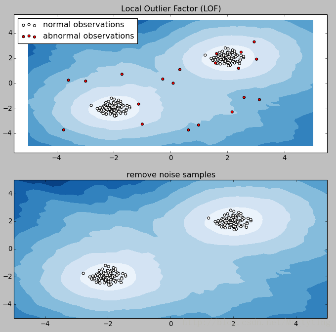
plt.show()显然在这个数据集中很好的去除了异常样本。
DBSCAN算法识别异常样本
可以利用聚类中的DBSCAN算法来检测异常,具体原理请看我的博文 机器学习–>无监督学习–>聚类里面相关介绍。#coding:utf-8 import numpy as np import matplotlib.pyplot as plt import sklearn.datasets as ds import matplotlib.colors from sklearn.cluster import DBSCAN from sklearn.preprocessing import StandardScaler def expand(a, b): d = (b - a) * 0.1 return a-d, b+d if __name__ == "__main__": N = 1000 centers = [[1, 2], [-1, -1], [1, -1], [-1, 1]] data, y = ds.make_blobs(N, n_features=2, centers=centers, cluster_std=[0.5, 0.25, 0.7, 0.5], random_state=0) data = StandardScaler().fit_transform(data) # 数据1的参数:(epsilon, min_sample) params = ((0.2, 5), (0.2, 10), (0.2, 15), (0.3, 5), (0.3, 10), (0.3, 15)) # 数据2 # t = np.arange(0, 2*np.pi, 0.1) # data1 = np.vstack((np.cos(t), np.sin(t))).T # data2 = np.vstack((2*np.cos(t), 2*np.sin(t))).T # data3 = np.vstack((3*np.cos(t), 3*np.sin(t))).T # data = np.vstack((data1, data2, data3)) # # # 数据2的参数:(epsilon, min_sample) # params = ((0.5, 3), (0.5, 5), (0.5, 10), (1., 3), (1., 10), (1., 20)) matplotlib.rcParams['font.sans-serif'] = [u'Droid Sans Fallback'] matplotlib.rcParams['axes.unicode_minus'] = False plt.figure(figsize=(12, 8), facecolor='w') plt.suptitle(u'DBSCAN聚类', fontsize=20) for i in range(6): eps, min_samples = params[i] model = DBSCAN(eps=eps, min_samples=min_samples) model.fit(data) y_hat = model.labels_ core_indices = np.zeros_like(y_hat, dtype=bool) core_indices[model.core_sample_indices_] = True y_unique = np.unique(y_hat) n_clusters = y_unique.size - (1 if -1 in y_hat else 0)## y_hat=-1为聚类后的噪声类 print y_unique, '聚类簇的个数为:', n_clusters plt.subplot(2, 3, i+1) clrs = plt.cm.Spectral(np.linspace(0, 0.8, y_unique.size))##指定聚类后每类的颜色 print clrs for k, clr in zip(y_unique, clrs): cur = (y_hat == k) if k == -1:##-1为异常样本 plt.scatter(data[cur, 0], data[cur, 1], s=20, c='black')## 画出异常样本点 continue plt.scatter(data[cur, 0], data[cur, 1], s=30, c=clr, edgecolors='k') #plt.scatter(data[cur & core_indices][:, 0], data[cur & core_indices][:, 1], s=60, c=clr, marker='o', edgecolors='k') x1_min, x2_min = np.min(data, axis=0) ## 两列的最小值 x1_max, x2_max = np.max(data, axis=0)## 两列的最大值 x1_min, x1_max = expand(x1_min, x1_max) x2_min, x2_max = expand(x2_min, x2_max) plt.xlim((x1_min, x1_max)) plt.ylim((x2_min, x2_max)) plt.grid(True) plt.title(ur'$\epsilon$ = %.1f m = %d,聚类数目:%d' % (eps, min_samples, n_clusters), fontsize=16) plt.tight_layout() plt.subplots_adjust(top=0.9) plt.show()
上述代码中,我们为DBSCAN选用了六组参数,画出在这六组参数下,对样本集聚类情况,并且识别出离群样本。离群样本为下图中的黑色原点。
在不同的参数下识别离群样本准备程度不一样。
那我们现在去掉这些识别出的黑色样本看看效果如何?
感觉清爽多了!并且有上图可以看出参数选择(0.2,15)时,聚类效果最好。
根据特征重要性检测异常样本
我们可以利用基于树的模型,比如xgboost,gbdt等训练模型得出特征的重要性排名,我们选取最重要的前k个特征,如果样本在这k个特征中缺失很多,那么我们可以认为这个样本是异常样本,是离群点。因为这个样本对整体模型的建立没有帮助,如果强行对其缺失值填充可能会引入噪声。
相关文章推荐
- 机器学习-->特征降维方法总结
- [Unity3D]引擎崩溃、异常、警告、BUG与提示总结及解决方法
- 基于PspCidTable的进程检测方法总结
- webdriver报不可见元素异常方法总结
- J2EE开发工作中遇到的异常问题及解决方法总结
- 目标检测方法总结(RFCN/SSD/RCNN/FastRCNN/FasterRCNN/SPPNet/DPM/OverFeat/YOLO)
- 阶段总结--业务系统代码中常见的异常错误总结以及避免方法
- 深度学习和机器学习最优化方法总结
- # include <errno.h >查看错误代码errno是调试程序的一个重要方法。当Linux C API函数发生异常时,一般会将errno变量赋值一个整数,不同的值表示不同的含义,可以通过查看
- 斯坦福大学(吴恩达) 机器学习课后习题详解 第九周 异常检测
- fckeditor异常总结---WARN No appenders could be found for logger的解决方法
- 机器学习优化方法总结比较(SGD,Adagrad,Adadelta,Adam,Adamax,Nadam)
- 《机器学习》第四章朴素贝叶斯分类器问题总结(python2.7->3.5)
- Android反调试方法总结以及源码实现之检测篇(一)
- js数据类型检测方法(总结)
- 机器学习第九周(一)--异常检测
- 角点检测方法总结
- 机器学习技法之Aggregation方法总结:Blending、Learning(Bagging、AdaBoost、Decision Tree)及其aggregation of aggregation
- Java一些常见的出错异常处理方法总结
- 机器学习公开课笔记(9):异常检测和推荐系统