Matlab 沿三维任意方向切割CT图的仿真计算
2017-06-25 20:29
295 查看

前言:本方法是为了解决一个实际医学场景而作。试想某患者头部插入异物,如何通过三维立体的方式显示出异物和头部组织的空间关系,为手术提供一定的参考。
一、数据来源
头部组织的数据。此处直接引用了matlab自带的mri数据。实际场景中,可以通过CT得到的数据进行转换得到插入异物的数据。此处我假设插入异物为一根细铁丝。模拟为空间中的一条曲线。这个曲线的坐标我们可以通过一定的办法获取到。我已经将数据放入百度云盘 曲线数据下载
二、实现要点
1. 要根据CT数据绘制头部的立体图2. 异物曲线的任意两点连线的切面的计算
3. 切面切割CT立体图的效果图绘制
三、实现代码第一部分
%% 数据准备
clc,clear
load mri;
D = squeeze(D);
D=double(D);
% img = importdata('image00.mat');
% c_start=1;
% D=img(:,:,:);
[m,n,q]=size(D);
%% 准备曲线数据
Curve = importdata('reference0.txt');
dataS=1000; %这两个参数 是我处理数据用的,数据太多,截取了一段曲线
dataLen=2000;
%
k=1; % 控制系数,让血管和脑补靠近
x_cur = (Curve(dataS:dataLen,1)/k);
y_cur = (Curve(dataS:dataLen,2)/k);
z_cur =-35+Curve(dataS:dataLen,3)/k;
figure
plot3(x_cur,y_cur,z_cur,'r*','linewidth',2)
title('单独曲线图')
grid on
xlabel('x');
ylabel('y');
zlabel('z');
grid on;
%为了画图方便
%画图
%%
%%
%另外还经常用到点法式方程:A(x-x0)+B(y-y0)+C(z-z0)=0
% x=x0+kt y=y0+mt z=z0+nt(x0,y0,z0)表示直线经过的一个点,t为任意实数,
% N_num=[100,200,300,400,500,600,700,800,900,1000];
% i=5;
% 而向量(k,m,n)表示直线的方向。
N=200; % 第多少个点;最好设置为100 200 300 ...1000.此处N 为控制切片位置的参数
x_start=x_cur(N-1);
y_start=y_cur(N-1);
z_start=z_cur(N-1);
x_end=x_cur(N+1);
y_end=y_cur(N+1);
z_end=z_cur(N+1);
x_mid=x_cur(N);
y_mid=y_cur(N);
z_mid=z_cur(N);
A=x_end-x_start;
B=y_end-y_start;
C=z_end-z_start;
x0=x_mid;
y0=y_mid;
z0=z_mid;
%%
%%生成与法线垂直的切片平面
[xs, ys] = meshgrid(0:1:128);
zs=-1*(((A*(xs-x_mid)+B*(ys-y_mid))./C)-z_mid);
[xxx,yyy,zzz]=meshgrid(1:m,1:n,1:q); %构造这个平面
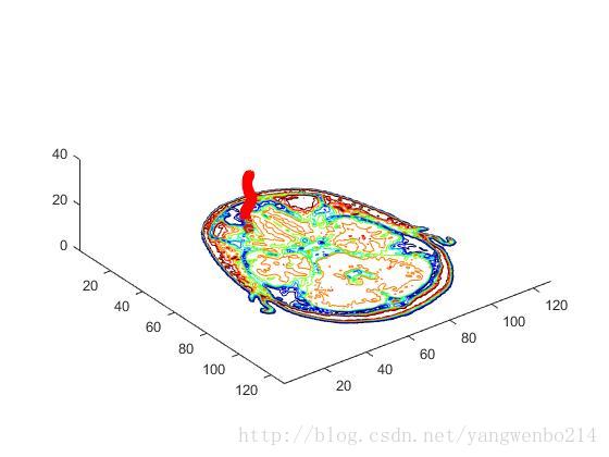
figure
plot3(x_cur,y_cur,z_cur,'r','linewidth',2)
xlabel('x');
ylabel('y');
zlabel('z');
grid on;
hold on;
slice(xxx,yyy,zzz,D,xs,ys,zs);
view(3)
shading interp
hold on调节N 的大小,可以得到一系列切割图。
四、实现代码第二部分(此段代码不注重切割方向):
如下代码直接和上述代码写在一起即可,第二部分代码有部分为参考他人的写法image_num=8;
image(D(:,:,image_num))%将矩阵D显示成图,D中每一个元素代表图像中一个长方形块的颜色
axis image%等同于axis equal设置宽高比使3个方向数据单位相同
x=xlim;%xlim返回当前x轴的界限
y=ylim;
cm=brighten(jet(length(map)),-.5);%使句柄为jet(length(map))的图形子对象变得更亮/暗 负为变暗
%jet, by itself, is the same length as the current figure's colormap. If no figure exists, MATLAB uses the length of the default colormap.
figure('Colormap',cm)
plot3(x_cur,y_cur,z_cur,'r*','linewidth',2)
hold on
contourslice(D,[],[],image_num)%在体积切平面中绘制等高线
axis ij%将坐标系的原点放在左上角
xlim(x)
ylim(y)
daspect([1,1,1])%设置轴数据的宽高比,此处设置x:y:z=1:1:1
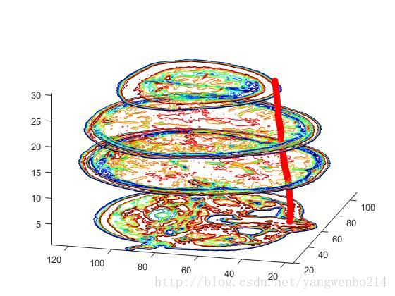
figure('Colormap',cm)
plot3(x_cur,y_cur,z_cur,'r*','linewidth',2)
hold on
contourslice(D,[1,2],[],[1,12,19,27],8);
view(3);%设置视角为默认的三维视图
axis tight%设置轴的限度为数据的范围效果图如下:
立体包络面展示
figure('Colormap',map)
plot3(x_cur,y_cur,z_cur,'r*','linewidth',2)
hold on
Ds=smooth3(D);%W = smooth3(V) smooths the input data V and returns the smoothed data in W.平滑输入数据D,输出Ds 变成double型数据
hiso = patch(isosurface(Ds,5),...%返回patch创建的块对象句柄;从块体数据中提取等值表面数据,返回等表面的面和顶点,可直接传递给patch;fv = isosurface(V,isovalue) assumes the arrays X, Y, and Z are defined as [X,Y,Z] = meshgrid(1:n,1:m,1:p) where [m,n,p] = size(V)
'FaceColor',[1,.75,.65],...
'EdgeColor','none');
isonormals(Ds,hiso)%计算等值表面顶点的法向 isonormals(V,p) and isonormals(X,Y,Z,V,p) set the VertexNormals property of the patch identified by the handle p to the computed normals rather than returning the values.

hcap=patch(isocaps(D,5),...%计算帽端等表面几何 D为块体数据 输出帽端的面、顶点和颜色数据给patch
'FaceColor','interp',...
'EdgeColor','none');

view(35,30)%两值设定了视角
axis tight
daspect([1,1,.4])

lightangle(45,30);%在球坐标系中创建并放置一个发光体,两值设定了视角lightangle(az,el) creates a light at the position specified by azimuth and elevation. az is the azimuthal (horizontal) rotation and el is the vertical elevation (both in degrees). The interpretation of azimuth and elevation is the same as that of the view command.
set(gcf,'Renderer','zbuffer');
lighting phong%指定冯氏明暗处理算法
set(hcap,'AmbientStrength',.6)
set(hiso,'SpecularColorReflectance',0,'SpecularExponent',50)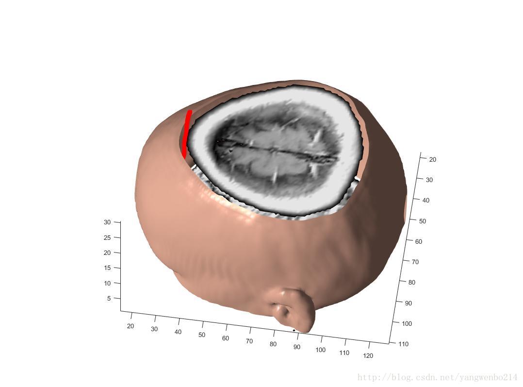

相关文章推荐
- Matlab:任意矩阵计算分布密度(海明距离的分布密度)
- Matlab投影仿真及三维曲面重构实现及演示程序
- 利用MATLAB计算三维坐标序列距离误差程序
- MATLAB BP神经网络中仿真结果与手工计算不符合的解决办法
- 利用MATLAB的GUI设计的一款可以进行FOCT电流比差计算的仿真平台
- 游戏里12方向,任意方向计算正前方矩形规则
- 三维场景计算任意两点的空间距离
- 三维软件开发笔记---任意方向切片完成
- 三维坐标点绕任意轴旋转的新坐标计算
- matlab实现炉温模糊控制器设计与仿真和PID控制器仿真比较详解_智能计算期末3
- 游戏里12方向,任意方向计算正前方矩形规则
- Matlab:任意矩阵计算分布密度(海明距离的分布密度)
- Matlab投影仿真及三维曲面重构实现及演示程序
- 流瞬ElectroMagneticWorks(EMWorks).EMS.2017.SP1.4.for.SW2011-2018.Win64三维电磁场仿真软件 EMS帮助设计人员计算的电、磁、机械和
- Matlab投影仿真及三维曲面重构实现及演示程序
- matlab计算任意多边形面积
- 三维坐标点绕任意轴旋转的新坐标计算
- 三维旋转矩阵(包括任意轴的通用旋转矩阵、Euler角、单位四元数)的计算
- 三维软件开发笔记---任意路径切割剖面完成
- MATLAB和C++数据交类实例---求任意函数y=f(x)的n阶导数,并计算在x=x0处的值