卡尔曼滤波器实例：跟踪自由落体运动：设计与Matlab实现

[首发：cnblogs 作者：byeyear Email：byeyear@hotmail.com]

本文所用实例来自于以下书籍：

Fundamentals of Kalman Filtering: A Practical Approach, 3rd Edition.Paul Zarchan, Howard Musoff.

某物体位于距地面400000 ft的高空，初速度为6000 ft/s，重力加速度为32.2 ft/s2。地面雷达位于其正下方测量该物体高度，测量周期0.1s，维持30s。已知雷达测量结果的标准差为1000 ft。

嗯，原书例子所用单位就是ft。与国标折算比例为0.3048。

取地面雷达位置为坐标原点，往上为正向。物理方程如下：

$x=400000-6000t-\frac{1}{2}gt^2$

从物理学的角度，选取距离、速度、加速度这三者作为系统状态是最直观的。将上式看做关于$t$的二阶多项式，其相应的状态转换矩阵和观测模型为：

$\boldsymbol{\Phi}_k = \left[ \begin{matrix} 1&T_s&0.5T_s^2 \\ 0&1&T_s \\ 0&0&1 \end{matrix} \right]$

$\mathbf{H} = \left[ \begin{matrix} 1&0&0 \end{matrix} \right]$

初始状态向量估计设为0，状态估计误差方差为$\infty$。

matlab程序如下：

order=3; % polynomial order is 3
ts=.1; % sample period
f2m=0.3048; % feet -> meter

t=[0:ts:30-ts];

s_init=400000*f2m; % init distance
v_init=-6000*f2m; % init speed
g_init=-9.8; % gravity
s=s_init + v_init .* t + 0.5 * g_init .* t .* t;
v=v_init + g_init .* t;
g=g_init * ones(1,300);
r=(1000*f2m)^2; % noise var
n=wgn(1, 300, r, 'linear');
sn=s+n; % signal with noise

x=zeros(3, 1); % init state vector
p=99999999999999 * eye(3,3); % estimate covariance
idn=eye(3); % unit matrix
phi=[1 ts 0.5*ts*ts; 0 1 ts; 0 0 1]; % fundmental matrix (p164)
h=[1 0 0];
phis=0; % no process noise
q=phis * [ts^5/20 ts^4/8 ts^3/6; ts^4/8 ts^3/3 ts^2/2; ts^3/6 ts^2/2 ts]; % but we still use q (p185)

xest=zeros(3,300);
xest_curr=zeros(3,1);

for i=[1:1:300]
xest_pre=phi*xest_curr;
p_pre = phi*p*phi'+q;
y=sn(:,i)-h*xest_pre;
ycov=h*p_pre*h'+r;
k=p_pre*h'*inv(ycov);
xest(:,i)=xest_pre+k*y;
p=(idn-k*h)*p_pre;
xest_curr=xest(:,i);
end

sest=zeros(1,300);
sest=h*xest;

plot(sest,'r');
hold on;
plot(s,'g');
hold on;
plot(sn,'b');
hold off;

执行结果如下图：







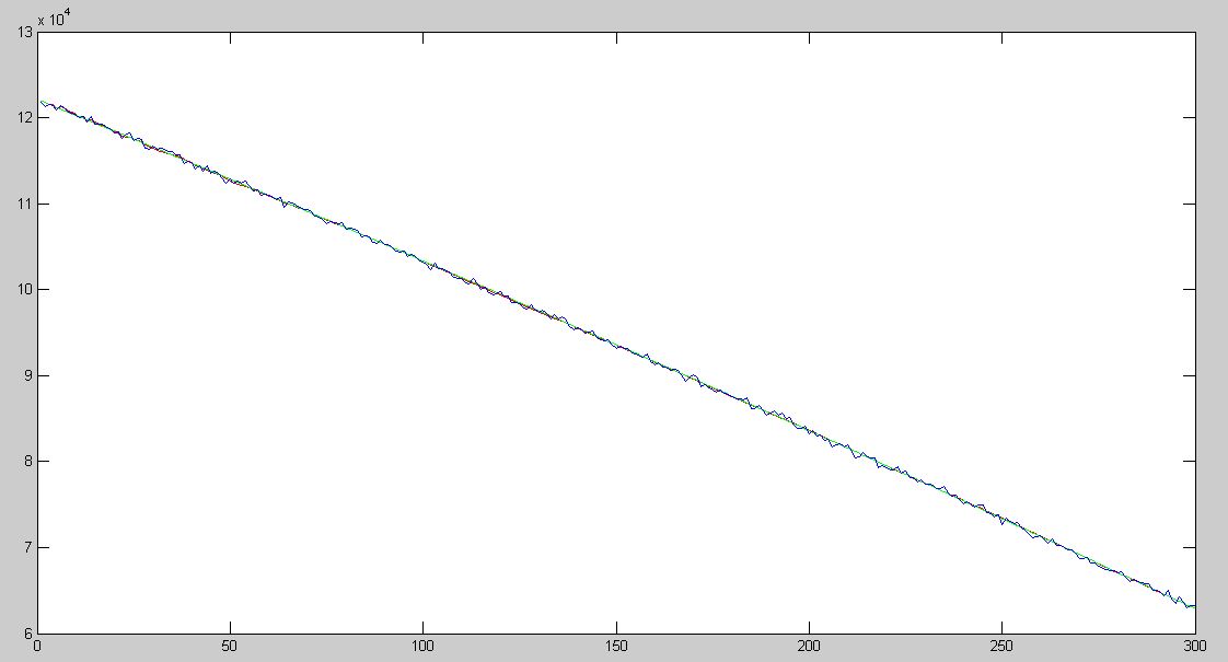
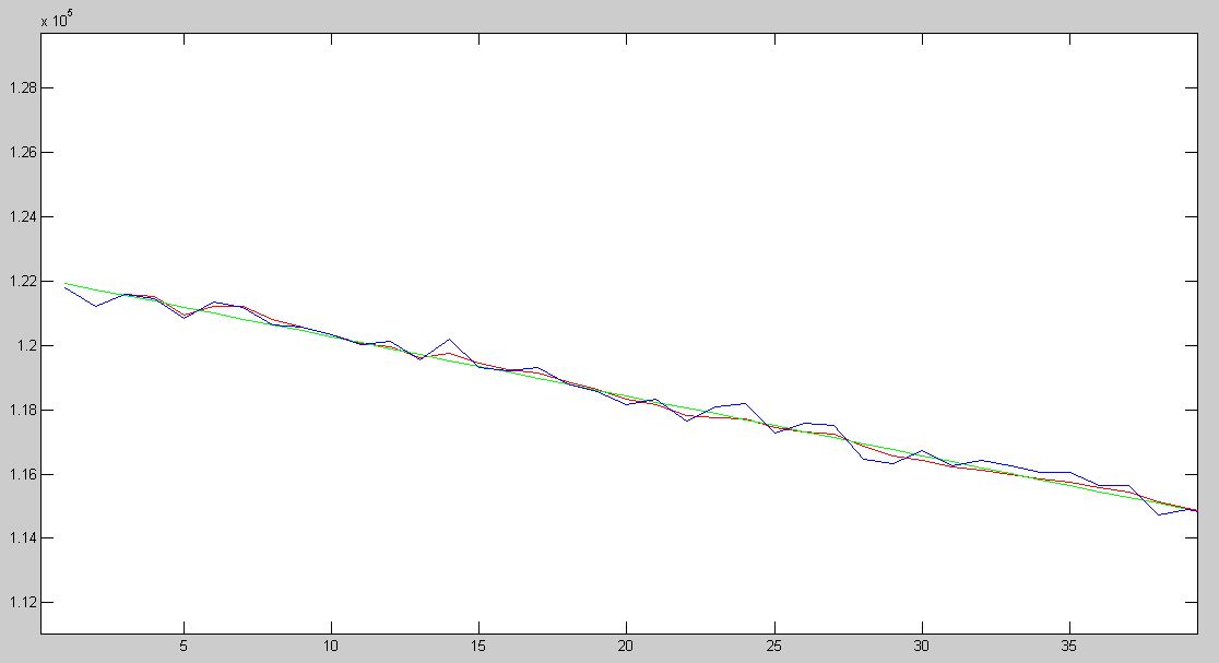
第一张图是全貌，看不出啥；

第二张图是开始约40个点，滤波器输出慢慢靠近理想值；

第三张图是最后约50个点，滤波器输出和理想值几乎重合。

下一次，我们将看到如何利用已知的重力加速度g，以一阶多项式的卡尔曼滤波器解决该问题。